
Dataset Viewer
prompt
stringlengths 501
4.98M
| target
stringclasses 1
value | chunk_prompt
bool 1
class | kind
stringclasses 2
values | prob
float64 0.2
0.97
⌀ | path
stringlengths 10
394
⌀ | quality_prob
float64 0.4
0.99
⌀ | learning_prob
float64 0.15
1
⌀ | filename
stringlengths 4
221
⌀ |
|---|---|---|---|---|---|---|---|---|
```
#export
from fastai.basics import *
from fastai.tabular.core import *
from fastai.tabular.model import *
from fastai.tabular.data import *
#hide
from nbdev.showdoc import *
#default_exp tabular.learner
```
# Tabular learner
> The function to immediately get a `Learner` ready to train for tabular data
The main function you probably want to use in this module is `tabular_learner`. It will automatically create a `TabulaModel` suitable for your data and infer the irght loss function. See the [tabular tutorial](http://docs.fast.ai/tutorial.tabular) for an example of use in context.
## Main functions
```
#export
@log_args(but_as=Learner.__init__)
class TabularLearner(Learner):
"`Learner` for tabular data"
def predict(self, row):
tst_to = self.dls.valid_ds.new(pd.DataFrame(row).T)
tst_to.process()
tst_to.conts = tst_to.conts.astype(np.float32)
dl = self.dls.valid.new(tst_to)
inp,preds,_,dec_preds = self.get_preds(dl=dl, with_input=True, with_decoded=True)
i = getattr(self.dls, 'n_inp', -1)
b = (*tuplify(inp),*tuplify(dec_preds))
full_dec = self.dls.decode((*tuplify(inp),*tuplify(dec_preds)))
return full_dec,dec_preds[0],preds[0]
show_doc(TabularLearner, title_level=3)
```
It works exactly as a normal `Learner`, the only difference is that it implements a `predict` method specific to work on a row of data.
```
#export
@log_args(to_return=True, but_as=Learner.__init__)
@delegates(Learner.__init__)
def tabular_learner(dls, layers=None, emb_szs=None, config=None, n_out=None, y_range=None, **kwargs):
"Get a `Learner` using `dls`, with `metrics`, including a `TabularModel` created using the remaining params."
if config is None: config = tabular_config()
if layers is None: layers = [200,100]
to = dls.train_ds
emb_szs = get_emb_sz(dls.train_ds, {} if emb_szs is None else emb_szs)
if n_out is None: n_out = get_c(dls)
assert n_out, "`n_out` is not defined, and could not be infered from data, set `dls.c` or pass `n_out`"
if y_range is None and 'y_range' in config: y_range = config.pop('y_range')
model = TabularModel(emb_szs, len(dls.cont_names), n_out, layers, y_range=y_range, **config)
return TabularLearner(dls, model, **kwargs)
```
If your data was built with fastai, you probably won't need to pass anything to `emb_szs` unless you want to change the default of the library (produced by `get_emb_sz`), same for `n_out` which should be automatically inferred. `layers` will default to `[200,100]` and is passed to `TabularModel` along with the `config`.
Use `tabular_config` to create a `config` and cusotmize the model used. There is just easy access to `y_range` because this argument is often used.
All the other arguments are passed to `Learner`.
```
path = untar_data(URLs.ADULT_SAMPLE)
df = pd.read_csv(path/'adult.csv')
cat_names = ['workclass', 'education', 'marital-status', 'occupation', 'relationship', 'race']
cont_names = ['age', 'fnlwgt', 'education-num']
procs = [Categorify, FillMissing, Normalize]
dls = TabularDataLoaders.from_df(df, path, procs=procs, cat_names=cat_names, cont_names=cont_names,
y_names="salary", valid_idx=list(range(800,1000)), bs=64)
learn = tabular_learner(dls)
#hide
tst = learn.predict(df.iloc[0])
#hide
#test y_range is passed
learn = tabular_learner(dls, y_range=(0,32))
assert isinstance(learn.model.layers[-1], SigmoidRange)
test_eq(learn.model.layers[-1].low, 0)
test_eq(learn.model.layers[-1].high, 32)
learn = tabular_learner(dls, config = tabular_config(y_range=(0,32)))
assert isinstance(learn.model.layers[-1], SigmoidRange)
test_eq(learn.model.layers[-1].low, 0)
test_eq(learn.model.layers[-1].high, 32)
#export
@typedispatch
def show_results(x:Tabular, y:Tabular, samples, outs, ctxs=None, max_n=10, **kwargs):
df = x.all_cols[:max_n]
for n in x.y_names: df[n+'_pred'] = y[n][:max_n].values
display_df(df)
```
## Export -
```
#hide
from nbdev.export import notebook2script
notebook2script()
```
| true |
code
| 0.704262 | null | null | null | null |
|
# Aerospike Connect for Spark - SparkML Prediction Model Tutorial
## Tested with Java 8, Spark 3.0.0, Python 3.7, and Aerospike Spark Connector 3.0.0
## Summary
Build a linear regression model to predict birth weight using Aerospike Database and Spark.
Here are the features used:
- gestation weeks
- mother’s age
- father’s age
- mother’s weight gain during pregnancy
- [Apgar score](https://en.wikipedia.org/wiki/Apgar_score)
Aerospike is used to store the Natality dataset that is published by CDC. The table is accessed in Apache Spark using the Aerospike Spark Connector, and Spark ML is used to build and evaluate the model. The model can later be converted to PMML and deployed on your inference server for predictions.
### Prerequisites
1. Load Aerospike server if not alrady available - docker run -d --name aerospike -p 3000:3000 -p 3001:3001 -p 3002:3002 -p 3003:3003 aerospike
2. Feature key needs to be located in AS_FEATURE_KEY_PATH
3. [Download the connector](https://www.aerospike.com/enterprise/download/connectors/aerospike-spark/3.0.0/)
```
#IP Address or DNS name for one host in your Aerospike cluster.
#A seed address for the Aerospike database cluster is required
AS_HOST ="127.0.0.1"
# Name of one of your namespaces. Type 'show namespaces' at the aql prompt if you are not sure
AS_NAMESPACE = "test"
AS_FEATURE_KEY_PATH = "/etc/aerospike/features.conf"
AEROSPIKE_SPARK_JAR_VERSION="3.0.0"
AS_PORT = 3000 # Usually 3000, but change here if not
AS_CONNECTION_STRING = AS_HOST + ":"+ str(AS_PORT)
#Locate the Spark installation - this'll use the SPARK_HOME environment variable
import findspark
findspark.init()
# Below will help you download the Spark Connector Jar if you haven't done so already.
import urllib
import os
def aerospike_spark_jar_download_url(version=AEROSPIKE_SPARK_JAR_VERSION):
DOWNLOAD_PREFIX="https://www.aerospike.com/enterprise/download/connectors/aerospike-spark/"
DOWNLOAD_SUFFIX="/artifact/jar"
AEROSPIKE_SPARK_JAR_DOWNLOAD_URL = DOWNLOAD_PREFIX+AEROSPIKE_SPARK_JAR_VERSION+DOWNLOAD_SUFFIX
return AEROSPIKE_SPARK_JAR_DOWNLOAD_URL
def download_aerospike_spark_jar(version=AEROSPIKE_SPARK_JAR_VERSION):
JAR_NAME="aerospike-spark-assembly-"+AEROSPIKE_SPARK_JAR_VERSION+".jar"
if(not(os.path.exists(JAR_NAME))) :
urllib.request.urlretrieve(aerospike_spark_jar_download_url(),JAR_NAME)
else :
print(JAR_NAME+" already downloaded")
return os.path.join(os.getcwd(),JAR_NAME)
AEROSPIKE_JAR_PATH=download_aerospike_spark_jar()
os.environ["PYSPARK_SUBMIT_ARGS"] = '--jars ' + AEROSPIKE_JAR_PATH + ' pyspark-shell'
import pyspark
from pyspark.context import SparkContext
from pyspark.sql.context import SQLContext
from pyspark.sql.session import SparkSession
from pyspark.ml.linalg import Vectors
from pyspark.ml.regression import LinearRegression
from pyspark.sql.types import StringType, StructField, StructType, ArrayType, IntegerType, MapType, LongType, DoubleType
#Get a spark session object and set required Aerospike configuration properties
sc = SparkContext.getOrCreate()
print("Spark Verison:", sc.version)
spark = SparkSession(sc)
sqlContext = SQLContext(sc)
spark.conf.set("aerospike.namespace",AS_NAMESPACE)
spark.conf.set("aerospike.seedhost",AS_CONNECTION_STRING)
spark.conf.set("aerospike.keyPath",AS_FEATURE_KEY_PATH )
```
## Step 1: Load Data into a DataFrame
```
as_data=spark \
.read \
.format("aerospike") \
.option("aerospike.set", "natality").load()
as_data.show(5)
print("Inferred Schema along with Metadata.")
as_data.printSchema()
```
### To speed up the load process at scale, use the [knobs](https://www.aerospike.com/docs/connect/processing/spark/performance.html) available in the Aerospike Spark Connector.
For example, **spark.conf.set("aerospike.partition.factor", 15 )** will map 4096 Aerospike partitions to 32K Spark partitions. <font color=red> (Note: Please configure this carefully based on the available resources (CPU threads) in your system.)</font>
## Step 2 - Prep data
```
# This Spark3.0 setting, if true, will turn on Adaptive Query Execution (AQE), which will make use of the
# runtime statistics to choose the most efficient query execution plan. It will speed up any joins that you
# plan to use for data prep step.
spark.conf.set("spark.sql.adaptive.enabled", 'true')
# Run a query in Spark SQL to ensure no NULL values exist.
as_data.createOrReplaceTempView("natality")
sql_query = """
SELECT *
from natality
where weight_pnd is not null
and mother_age is not null
and father_age is not null
and father_age < 80
and gstation_week is not null
and weight_gain_pnd < 90
and apgar_5min != "99"
and apgar_5min != "88"
"""
clean_data = spark.sql(sql_query)
#Drop the Aerospike metadata from the dataset because its not required.
#The metadata is added because we are inferring the schema as opposed to providing a strict schema
columns_to_drop = ['__key','__digest','__expiry','__generation','__ttl' ]
clean_data = clean_data.drop(*columns_to_drop)
# dropping null values
clean_data = clean_data.dropna()
clean_data.cache()
clean_data.show(5)
#Descriptive Analysis of the data
clean_data.describe().toPandas().transpose()
```
## Step 3 Visualize Data
```
import numpy as np
import matplotlib.pyplot as plt
import pandas as pd
import math
pdf = clean_data.toPandas()
#Histogram - Father Age
pdf[['father_age']].plot(kind='hist',bins=10,rwidth=0.8)
plt.xlabel('Fathers Age (years)',fontsize=12)
plt.legend(loc=None)
plt.style.use('seaborn-whitegrid')
plt.show()
'''
pdf[['mother_age']].plot(kind='hist',bins=10,rwidth=0.8)
plt.xlabel('Mothers Age (years)',fontsize=12)
plt.legend(loc=None)
plt.style.use('seaborn-whitegrid')
plt.show()
'''
pdf[['weight_pnd']].plot(kind='hist',bins=10,rwidth=0.8)
plt.xlabel('Babys Weight (Pounds)',fontsize=12)
plt.legend(loc=None)
plt.style.use('seaborn-whitegrid')
plt.show()
pdf[['gstation_week']].plot(kind='hist',bins=10,rwidth=0.8)
plt.xlabel('Gestation (Weeks)',fontsize=12)
plt.legend(loc=None)
plt.style.use('seaborn-whitegrid')
plt.show()
pdf[['weight_gain_pnd']].plot(kind='hist',bins=10,rwidth=0.8)
plt.xlabel('mother’s weight gain during pregnancy',fontsize=12)
plt.legend(loc=None)
plt.style.use('seaborn-whitegrid')
plt.show()
#Histogram - Apgar Score
print("Apgar Score: Scores of 7 and above are generally normal; 4 to 6, fairly low; and 3 and below are generally \
regarded as critically low and cause for immediate resuscitative efforts.")
pdf[['apgar_5min']].plot(kind='hist',bins=10,rwidth=0.8)
plt.xlabel('Apgar score',fontsize=12)
plt.legend(loc=None)
plt.style.use('seaborn-whitegrid')
plt.show()
```
## Step 4 - Create Model
**Steps used for model creation:**
1. Split cleaned data into Training and Test sets
2. Vectorize features on which the model will be trained
3. Create a linear regression model (Choose any ML algorithm that provides the best fit for the given dataset)
4. Train model (Although not shown here, you could use K-fold cross-validation and Grid Search to choose the best hyper-parameters for the model)
5. Evaluate model
```
# Define a function that collects the features of interest
# (mother_age, father_age, and gestation_weeks) into a vector.
# Package the vector in a tuple containing the label (`weight_pounds`) for that
# row.##
def vector_from_inputs(r):
return (r["weight_pnd"], Vectors.dense(float(r["mother_age"]),
float(r["father_age"]),
float(r["gstation_week"]),
float(r["weight_gain_pnd"]),
float(r["apgar_5min"])))
#Split that data 70% training and 30% Evaluation data
train, test = clean_data.randomSplit([0.7, 0.3])
#Check the shape of the data
train.show()
print((train.count(), len(train.columns)))
test.show()
print((test.count(), len(test.columns)))
# Create an input DataFrame for Spark ML using the above function.
training_data = train.rdd.map(vector_from_inputs).toDF(["label",
"features"])
# Construct a new LinearRegression object and fit the training data.
lr = LinearRegression(maxIter=5, regParam=0.2, solver="normal")
#Voila! your first model using Spark ML is trained
model = lr.fit(training_data)
# Print the model summary.
print("Coefficients:" + str(model.coefficients))
print("Intercept:" + str(model.intercept))
print("R^2:" + str(model.summary.r2))
model.summary.residuals.show()
```
### Evaluate Model
```
eval_data = test.rdd.map(vector_from_inputs).toDF(["label",
"features"])
eval_data.show()
evaluation_summary = model.evaluate(eval_data)
print("MAE:", evaluation_summary.meanAbsoluteError)
print("RMSE:", evaluation_summary.rootMeanSquaredError)
print("R-squared value:", evaluation_summary.r2)
```
## Step 5 - Batch Prediction
```
#eval_data contains the records (ideally production) that you'd like to use for the prediction
predictions = model.transform(eval_data)
predictions.show()
```
#### Compare the labels and the predictions, they should ideally match up for an accurate model. Label is the actual weight of the baby and prediction is the predicated weight
### Saving the Predictions to Aerospike for ML Application's consumption
```
# Aerospike is a key/value database, hence a key is needed to store the predictions into the database. Hence we need
# to add the _id column to the predictions using SparkSQL
predictions.createOrReplaceTempView("predict_view")
sql_query = """
SELECT *, monotonically_increasing_id() as _id
from predict_view
"""
predict_df = spark.sql(sql_query)
predict_df.show()
print("#records:", predict_df.count())
# Now we are good to write the Predictions to Aerospike
predict_df \
.write \
.mode('overwrite') \
.format("aerospike") \
.option("aerospike.writeset", "predictions")\
.option("aerospike.updateByKey", "_id") \
.save()
```
#### You can verify that data is written to Aerospike by using either [AQL](https://www.aerospike.com/docs/tools/aql/data_management.html) or the [Aerospike Data Browser](https://github.com/aerospike/aerospike-data-browser)
## Step 6 - Deploy
### Here are a few options:
1. Save the model to a PMML file by converting it using Jpmml/[pyspark2pmml](https://github.com/jpmml/pyspark2pmml) and load it into your production enviornment for inference.
2. Use Aerospike as an [edge database for high velocity ingestion](https://medium.com/aerospike-developer-blog/add-horsepower-to-ai-ml-pipeline-15ca42a10982) for your inference pipline.
| true |
code
| 0.475301 | null | null | null | null |
|
# Classification on Iris dataset with sklearn and DJL
In this notebook, you will try to use a pre-trained sklearn model to run on DJL for a general classification task. The model was trained with [Iris flower dataset](https://en.wikipedia.org/wiki/Iris_flower_data_set).
## Background
### Iris Dataset
The dataset contains a set of 150 records under five attributes - sepal length, sepal width, petal length, petal width and species.
Iris setosa | Iris versicolor | Iris virginica
:-------------------------:|:-------------------------:|:-------------------------:
 |  | 
The chart above shows three different kinds of the Iris flowers.
We will use sepal length, sepal width, petal length, petal width as the feature and species as the label to train the model.
### Sklearn Model
You can find more information [here](http://onnx.ai/sklearn-onnx/). You can use the sklearn built-in iris dataset to load the data. Then we defined a [RandomForestClassifer](https://scikit-learn.org/stable/modules/generated/sklearn.ensemble.RandomForestClassifier.html) to train the model. After that, we convert the model to onnx format for DJL to run inference. The following code is a sample classification setup using sklearn:
```python
# Train a model.
from sklearn.datasets import load_iris
from sklearn.model_selection import train_test_split
from sklearn.ensemble import RandomForestClassifier
iris = load_iris()
X, y = iris.data, iris.target
X_train, X_test, y_train, y_test = train_test_split(X, y)
clr = RandomForestClassifier()
clr.fit(X_train, y_train)
```
## Preparation
This tutorial requires the installation of Java Kernel. To install the Java Kernel, see the [README](https://github.com/awslabs/djl/blob/master/jupyter/README.md).
These are dependencies we will use. To enhance the NDArray operation capability, we are importing ONNX Runtime and PyTorch Engine at the same time. Please find more information [here](https://github.com/awslabs/djl/blob/master/docs/onnxruntime/hybrid_engine.md#hybrid-engine-for-onnx-runtime).
```
// %mavenRepo snapshots https://oss.sonatype.org/content/repositories/snapshots/
%maven ai.djl:api:0.8.0
%maven ai.djl.onnxruntime:onnxruntime-engine:0.8.0
%maven ai.djl.pytorch:pytorch-engine:0.8.0
%maven org.slf4j:slf4j-api:1.7.26
%maven org.slf4j:slf4j-simple:1.7.26
%maven com.microsoft.onnxruntime:onnxruntime:1.4.0
%maven ai.djl.pytorch:pytorch-native-auto:1.6.0
import ai.djl.inference.*;
import ai.djl.modality.*;
import ai.djl.ndarray.*;
import ai.djl.ndarray.types.*;
import ai.djl.repository.zoo.*;
import ai.djl.translate.*;
import java.util.*;
```
## Step 1 create a Translator
Inference in machine learning is the process of predicting the output for a given input based on a pre-defined model.
DJL abstracts away the whole process for ease of use. It can load the model, perform inference on the input, and provide
output. DJL also allows you to provide user-defined inputs. The workflow looks like the following:
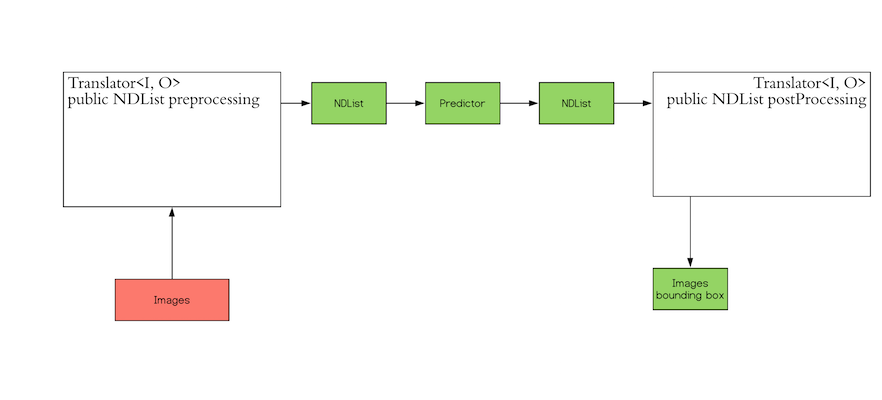
The `Translator` interface encompasses the two white blocks: Pre-processing and Post-processing. The pre-processing
component converts the user-defined input objects into an NDList, so that the `Predictor` in DJL can understand the
input and make its prediction. Similarly, the post-processing block receives an NDList as the output from the
`Predictor`. The post-processing block allows you to convert the output from the `Predictor` to the desired output
format.
In our use case, we use a class namely `IrisFlower` as our input class type. We will use [`Classifications`](https://javadoc.io/doc/ai.djl/api/latest/ai/djl/modality/Classifications.html) as our output class type.
```
public static class IrisFlower {
public float sepalLength;
public float sepalWidth;
public float petalLength;
public float petalWidth;
public IrisFlower(float sepalLength, float sepalWidth, float petalLength, float petalWidth) {
this.sepalLength = sepalLength;
this.sepalWidth = sepalWidth;
this.petalLength = petalLength;
this.petalWidth = petalWidth;
}
}
```
Let's create a translator
```
public static class MyTranslator implements Translator<IrisFlower, Classifications> {
private final List<String> synset;
public MyTranslator() {
// species name
synset = Arrays.asList("setosa", "versicolor", "virginica");
}
@Override
public NDList processInput(TranslatorContext ctx, IrisFlower input) {
float[] data = {input.sepalLength, input.sepalWidth, input.petalLength, input.petalWidth};
NDArray array = ctx.getNDManager().create(data, new Shape(1, 4));
return new NDList(array);
}
@Override
public Classifications processOutput(TranslatorContext ctx, NDList list) {
return new Classifications(synset, list.get(1));
}
@Override
public Batchifier getBatchifier() {
return null;
}
}
```
## Step 2 Prepare your model
We will load a pretrained sklearn model into DJL. We defined a [`ModelZoo`](https://javadoc.io/doc/ai.djl/api/latest/ai/djl/repository/zoo/ModelZoo.html) concept to allow user load model from varity of locations, such as remote URL, local files or DJL pretrained model zoo. We need to define `Criteria` class to help the modelzoo locate the model and attach translator. In this example, we download a compressed ONNX model from S3.
```
String modelUrl = "https://mlrepo.djl.ai/model/tabular/random_forest/ai/djl/onnxruntime/iris_flowers/0.0.1/iris_flowers.zip";
Criteria<IrisFlower, Classifications> criteria = Criteria.builder()
.setTypes(IrisFlower.class, Classifications.class)
.optModelUrls(modelUrl)
.optTranslator(new MyTranslator())
.optEngine("OnnxRuntime") // use OnnxRuntime engine by default
.build();
ZooModel<IrisFlower, Classifications> model = ModelZoo.loadModel(criteria);
```
## Step 3 Run inference
User will just need to create a `Predictor` from model to run the inference.
```
Predictor<IrisFlower, Classifications> predictor = model.newPredictor();
IrisFlower info = new IrisFlower(1.0f, 2.0f, 3.0f, 4.0f);
predictor.predict(info);
```
| true |
code
| 0.782642 | null | null | null | null |
|
<a href="https://colab.research.google.com/github/satyajitghana/TSAI-DeepNLP-END2.0/blob/main/09_NLP_Evaluation/ClassificationEvaluation.ipynb" target="_parent"><img src="https://colab.research.google.com/assets/colab-badge.svg" alt="Open In Colab"/></a>
```
! pip3 install git+https://github.com/extensive-nlp/ttc_nlp --quiet
! pip3 install torchmetrics --quiet
from ttctext.datamodules.sst import SSTDataModule
from ttctext.datasets.sst import StanfordSentimentTreeBank
sst_dataset = SSTDataModule(batch_size=128)
sst_dataset.setup()
import pytorch_lightning as pl
import torch
import torch.nn as nn
import torch.nn.functional as F
from torchmetrics.functional import accuracy, precision, recall, confusion_matrix
from sklearn.metrics import classification_report
import matplotlib.pyplot as plt
import seaborn as sns
import pandas as pd
sns.set()
class SSTModel(pl.LightningModule):
def __init__(self, hparams, *args, **kwargs):
super().__init__()
self.save_hyperparameters(hparams)
self.num_classes = self.hparams.output_dim
self.embedding = nn.Embedding(self.hparams.input_dim, self.hparams.embedding_dim)
self.lstm = nn.LSTM(
self.hparams.embedding_dim,
self.hparams.hidden_dim,
num_layers=self.hparams.num_layers,
dropout=self.hparams.dropout,
batch_first=True
)
self.proj_layer = nn.Sequential(
nn.Linear(self.hparams.hidden_dim, self.hparams.hidden_dim),
nn.BatchNorm1d(self.hparams.hidden_dim),
nn.ReLU(),
nn.Dropout(self.hparams.dropout),
)
self.fc = nn.Linear(self.hparams.hidden_dim, self.num_classes)
self.loss = nn.CrossEntropyLoss()
def init_state(self, sequence_length):
return (torch.zeros(self.hparams.num_layers, sequence_length, self.hparams.hidden_dim).to(self.device),
torch.zeros(self.hparams.num_layers, sequence_length, self.hparams.hidden_dim).to(self.device))
def forward(self, text, text_length, prev_state=None):
# [batch size, sentence length] => [batch size, sentence len, embedding size]
embedded = self.embedding(text)
# packs the input for faster forward pass in RNN
packed = torch.nn.utils.rnn.pack_padded_sequence(
embedded, text_length.to('cpu'),
enforce_sorted=False,
batch_first=True
)
# [batch size sentence len, embedding size] =>
# output: [batch size, sentence len, hidden size]
# hidden: [batch size, 1, hidden size]
packed_output, curr_state = self.lstm(packed, prev_state)
hidden_state, cell_state = curr_state
# print('hidden state shape: ', hidden_state.shape)
# print('cell')
# unpack packed sequence
# unpacked, unpacked_len = torch.nn.utils.rnn.pad_packed_sequence(packed_output, batch_first=True)
# print('unpacked: ', unpacked.shape)
# [batch size, sentence len, hidden size] => [batch size, num classes]
# output = self.proj_layer(unpacked[:, -1])
output = self.proj_layer(hidden_state[-1])
# print('output shape: ', output.shape)
output = self.fc(output)
return output, curr_state
def shared_step(self, batch, batch_idx):
label, text, text_length = batch
logits, in_state = self(text, text_length)
loss = self.loss(logits, label)
pred = torch.argmax(F.log_softmax(logits, dim=1), dim=1)
acc = accuracy(pred, label)
metric = {'loss': loss, 'acc': acc, 'pred': pred, 'label': label}
return metric
def training_step(self, batch, batch_idx):
metrics = self.shared_step(batch, batch_idx)
log_metrics = {'train_loss': metrics['loss'], 'train_acc': metrics['acc']}
self.log_dict(log_metrics, prog_bar=True)
return metrics
def validation_step(self, batch, batch_idx):
metrics = self.shared_step(batch, batch_idx)
return metrics
def validation_epoch_end(self, outputs):
acc = torch.stack([x['acc'] for x in outputs]).mean()
loss = torch.stack([x['loss'] for x in outputs]).mean()
log_metrics = {'val_loss': loss, 'val_acc': acc}
self.log_dict(log_metrics, prog_bar=True)
if self.trainer.sanity_checking:
return log_metrics
preds = torch.cat([x['pred'] for x in outputs]).view(-1)
labels = torch.cat([x['label'] for x in outputs]).view(-1)
accuracy_ = accuracy(preds, labels)
precision_ = precision(preds, labels, average='macro', num_classes=self.num_classes)
recall_ = recall(preds, labels, average='macro', num_classes=self.num_classes)
classification_report_ = classification_report(labels.cpu().numpy(), preds.cpu().numpy(), target_names=self.hparams.class_labels)
confusion_matrix_ = confusion_matrix(preds, labels, num_classes=self.num_classes)
cm_df = pd.DataFrame(confusion_matrix_.cpu().numpy(), index=self.hparams.class_labels, columns=self.hparams.class_labels)
print(f'Test Epoch {self.current_epoch}/{self.hparams.epochs-1}: F1 Score: {accuracy_:.5f}, Precision: {precision_:.5f}, Recall: {recall_:.5f}\n')
print(f'Classification Report\n{classification_report_}')
fig, ax = plt.subplots(figsize=(10, 8))
heatmap = sns.heatmap(cm_df, annot=True, ax=ax, fmt='d') # font size
locs, labels = plt.xticks()
plt.setp(labels, rotation=45)
locs, labels = plt.yticks()
plt.setp(labels, rotation=45)
plt.show()
print("\n")
return log_metrics
def test_step(self, batch, batch_idx):
return self.validation_step(batch, batch_idx)
def test_epoch_end(self, outputs):
accuracy = torch.stack([x['acc'] for x in outputs]).mean()
self.log('hp_metric', accuracy)
self.log_dict({'test_acc': accuracy}, prog_bar=True)
def configure_optimizers(self):
optimizer = torch.optim.Adam(self.parameters(), lr=self.hparams.lr)
lr_scheduler = {
'scheduler': torch.optim.lr_scheduler.ReduceLROnPlateau(optimizer, patience=10, verbose=True),
'monitor': 'train_loss',
'name': 'scheduler'
}
return [optimizer], [lr_scheduler]
from omegaconf import OmegaConf
hparams = OmegaConf.create({
'input_dim': len(sst_dataset.get_vocab()),
'embedding_dim': 128,
'num_layers': 2,
'hidden_dim': 64,
'dropout': 0.5,
'output_dim': len(StanfordSentimentTreeBank.get_labels()),
'class_labels': sst_dataset.raw_dataset_train.get_labels(),
'lr': 5e-4,
'epochs': 10,
'use_lr_finder': False
})
sst_model = SSTModel(hparams)
trainer = pl.Trainer(gpus=1, max_epochs=hparams.epochs, progress_bar_refresh_rate=1, reload_dataloaders_every_epoch=True)
trainer.fit(sst_model, sst_dataset)
```
| true |
code
| 0.862265 | null | null | null | null |
|
## Accessing TerraClimate data with the Planetary Computer STAC API
[TerraClimate](http://www.climatologylab.org/terraclimate.html) is a dataset of monthly climate and climatic water balance for global terrestrial surfaces from 1958-2019. These data provide important inputs for ecological and hydrological studies at global scales that require high spatial resolution and time-varying data. All data have monthly temporal resolution and a ~4-km (1/24th degree) spatial resolution. The data cover the period from 1958-2019.
This example will show you how temperature has increased over the past 60 years across the globe.
### Environment setup
```
import warnings
warnings.filterwarnings("ignore", "invalid value", RuntimeWarning)
```
### Data access
https://planetarycomputer.microsoft.com/api/stac/v1/collections/terraclimate is a STAC Collection with links to all the metadata about this dataset. We'll load it with [PySTAC](https://pystac.readthedocs.io/en/latest/).
```
import pystac
url = "https://planetarycomputer.microsoft.com/api/stac/v1/collections/terraclimate"
collection = pystac.read_file(url)
collection
```
The collection contains assets, which are links to the root of a Zarr store, which can be opened with xarray.
```
asset = collection.assets["zarr-https"]
asset
import fsspec
import xarray as xr
store = fsspec.get_mapper(asset.href)
ds = xr.open_zarr(store, **asset.extra_fields["xarray:open_kwargs"])
ds
```
We'll process the data in parallel using [Dask](https://dask.org).
```
from dask_gateway import GatewayCluster
cluster = GatewayCluster()
cluster.scale(16)
client = cluster.get_client()
print(cluster.dashboard_link)
```
The link printed out above can be opened in a new tab or the [Dask labextension](https://github.com/dask/dask-labextension). See [Scale with Dask](https://planetarycomputer.microsoft.com/docs/quickstarts/scale-with-dask/) for more on using Dask, and how to access the Dashboard.
### Analyze and plot global temperature
We can quickly plot a map of one of the variables. In this case, we are downsampling (coarsening) the dataset for easier plotting.
```
import cartopy.crs as ccrs
import matplotlib.pyplot as plt
average_max_temp = ds.isel(time=-1)["tmax"].coarsen(lat=8, lon=8).mean().load()
fig, ax = plt.subplots(figsize=(20, 10), subplot_kw=dict(projection=ccrs.Robinson()))
average_max_temp.plot(ax=ax, transform=ccrs.PlateCarree())
ax.coastlines();
```
Let's see how temperature has changed over the observational record, when averaged across the entire domain. Since we'll do some other calculations below we'll also add `.load()` to execute the command instead of specifying it lazily. Note that there are some data quality issues before 1965 so we'll start our analysis there.
```
temperature = (
ds["tmax"].sel(time=slice("1965", None)).mean(dim=["lat", "lon"]).persist()
)
temperature.plot(figsize=(12, 6));
```
With all the seasonal fluctuations (from summer and winter) though, it can be hard to see any obvious trends. So let's try grouping by year and plotting that timeseries.
```
temperature.groupby("time.year").mean().plot(figsize=(12, 6));
```
Now the increase in temperature is obvious, even when averaged across the entire domain.
Now, let's see how those changes are different in different parts of the world. And let's focus just on summer months in the northern hemisphere, when it's hottest. Let's take a climatological slice at the beginning of the period and the same at the end of the period, calculate the difference, and map it to see how different parts of the world have changed differently.
First we'll just grab the summer months.
```
%%time
import dask
summer_months = [6, 7, 8]
summer = ds.tmax.where(ds.time.dt.month.isin(summer_months), drop=True)
early_period = slice("1958-01-01", "1988-12-31")
late_period = slice("1988-01-01", "2018-12-31")
early, late = dask.compute(
summer.sel(time=early_period).mean(dim="time"),
summer.sel(time=late_period).mean(dim="time"),
)
increase = (late - early).coarsen(lat=8, lon=8).mean()
fig, ax = plt.subplots(figsize=(20, 10), subplot_kw=dict(projection=ccrs.Robinson()))
increase.plot(ax=ax, transform=ccrs.PlateCarree(), robust=True)
ax.coastlines();
```
This shows us that changes in summer temperature haven't been felt equally around the globe. Note the enhanced warming in the polar regions, a phenomenon known as "Arctic amplification".
| true |
code
| 0.609059 | null | null | null | null |
|
```
import numpy as np
import matplotlib.pyplot as plt
import numba
from tqdm import tqdm
import eitest
```
# Data generators
```
@numba.njit
def event_series_bernoulli(series_length, event_count):
'''Generate an iid Bernoulli distributed event series.
series_length: length of the event series
event_count: number of events'''
event_series = np.zeros(series_length)
event_series[np.random.choice(np.arange(0, series_length), event_count, replace=False)] = 1
return event_series
@numba.njit
def time_series_mean_impact(event_series, order, signal_to_noise):
'''Generate a time series with impacts in mean as described in the paper.
The impact weights are sampled iid from N(0, signal_to_noise),
and additional noise is sampled iid from N(0,1). The detection problem will
be harder than in time_series_meanconst_impact for small orders, as for small
orders we have a low probability to sample at least one impact weight with a
high magnitude. On the other hand, since the impact is different at every lag,
we can detect the impacts even if the order is larger than the max_lag value
used in the test.
event_series: input of shape (T,) with event occurrences
order: order of the event impacts
signal_to_noise: signal to noise ratio of the event impacts'''
series_length = len(event_series)
weights = np.random.randn(order)*np.sqrt(signal_to_noise)
time_series = np.random.randn(series_length)
for t in range(series_length):
if event_series[t] == 1:
time_series[t+1:t+order+1] += weights[:order-max(0, (t+order+1)-series_length)]
return time_series
@numba.njit
def time_series_meanconst_impact(event_series, order, const):
'''Generate a time series with impacts in mean by adding a constant.
Better for comparing performance across different impact orders, since the
magnitude of the impact will always be the same.
event_series: input of shape (T,) with event occurrences
order: order of the event impacts
const: constant for mean shift'''
series_length = len(event_series)
time_series = np.random.randn(series_length)
for t in range(series_length):
if event_series[t] == 1:
time_series[t+1:t+order+1] += const
return time_series
@numba.njit
def time_series_var_impact(event_series, order, variance):
'''Generate a time series with impacts in variance as described in the paper.
event_series: input of shape (T,) with event occurrences
order: order of the event impacts
variance: variance under event impacts'''
series_length = len(event_series)
time_series = np.random.randn(series_length)
for t in range(series_length):
if event_series[t] == 1:
for tt in range(t+1, min(series_length, t+order+1)):
time_series[tt] = np.random.randn()*np.sqrt(variance)
return time_series
@numba.njit
def time_series_tail_impact(event_series, order, dof):
'''Generate a time series with impacts in tails as described in the paper.
event_series: input of shape (T,) with event occurrences
order: delay of the event impacts
dof: degrees of freedom of the t distribution'''
series_length = len(event_series)
time_series = np.random.randn(series_length)*np.sqrt(dof/(dof-2))
for t in range(series_length):
if event_series[t] == 1:
for tt in range(t+1, min(series_length, t+order+1)):
time_series[tt] = np.random.standard_t(dof)
return time_series
```
# Visualization of the impact models
```
default_T = 8192
default_N = 64
default_q = 4
es = event_series_bernoulli(default_T, default_N)
for ts in [
time_series_mean_impact(es, order=default_q, signal_to_noise=10.),
time_series_meanconst_impact(es, order=default_q, const=5.),
time_series_var_impact(es, order=default_q, variance=4.),
time_series_tail_impact(es, order=default_q, dof=3.),
]:
fig, (ax1, ax2) = plt.subplots(1, 2, gridspec_kw={'width_ratios': [2, 1]}, figsize=(15, 2))
ax1.plot(ts)
ax1.plot(es*np.max(ts), alpha=0.5)
ax1.set_xlim(0, len(es))
samples = eitest.obtain_samples(es, ts, method='eager', lag_cutoff=15, instantaneous=True)
eitest.plot_samples(samples, ax2)
plt.show()
```
# Simulations
```
def test_simul_pairs(impact_model, param_T, param_N, param_q, param_r,
n_pairs, lag_cutoff, instantaneous, sample_method,
twosamp_test, multi_test, alpha):
true_positive = 0.
false_positive = 0.
for _ in tqdm(range(n_pairs)):
es = event_series_bernoulli(param_T, param_N)
if impact_model == 'mean':
ts = time_series_mean_impact(es, param_q, param_r)
elif impact_model == 'meanconst':
ts = time_series_meanconst_impact(es, param_q, param_r)
elif impact_model == 'var':
ts = time_series_var_impact(es, param_q, param_r)
elif impact_model == 'tail':
ts = time_series_tail_impact(es, param_q, param_r)
else:
raise ValueError('impact_model must be "mean", "meanconst", "var" or "tail"')
# coupled pair
samples = eitest.obtain_samples(es, ts, lag_cutoff=lag_cutoff,
method=sample_method,
instantaneous=instantaneous,
sort=(twosamp_test == 'ks')) # samples need to be sorted for K-S test
tstats, pvals = eitest.pairwise_twosample_tests(samples, twosamp_test, min_pts=2)
pvals_adj = eitest.multitest(np.sort(pvals[~np.isnan(pvals)]), multi_test)
true_positive += (pvals_adj.min() < alpha)
# uncoupled pair
samples = eitest.obtain_samples(np.random.permutation(es), ts, lag_cutoff=lag_cutoff,
method=sample_method,
instantaneous=instantaneous,
sort=(twosamp_test == 'ks'))
tstats, pvals = eitest.pairwise_twosample_tests(samples, twosamp_test, min_pts=2)
pvals_adj = eitest.multitest(np.sort(pvals[~np.isnan(pvals)]), multi_test)
false_positive += (pvals_adj.min() < alpha)
return true_positive/n_pairs, false_positive/n_pairs
# global parameters
default_T = 8192
n_pairs = 100
alpha = 0.05
twosamp_test = 'ks'
multi_test = 'simes'
sample_method = 'lazy'
lag_cutoff = 32
instantaneous = True
```
## Mean impact model
```
default_N = 64
default_r = 1.
default_q = 4
```
### ... by number of events
```
vals = [4, 8, 16, 32, 64, 128, 256]
tprs = np.empty(len(vals))
fprs = np.empty(len(vals))
for i, val in enumerate(vals):
tprs[i], fprs[i] = test_simul_pairs(impact_model='mean', param_T=default_T,
param_N=val, param_q=default_q, param_r=default_r,
n_pairs=n_pairs, sample_method=sample_method,
lag_cutoff=lag_cutoff, instantaneous=instantaneous,
twosamp_test=twosamp_test, multi_test=multi_test, alpha=alpha)
plt.figure(figsize=(3,3))
plt.axvline(default_N, ls='-', c='gray', lw=1, label='def')
plt.axhline(alpha, ls='--', c='black', lw=1, label='alpha')
plt.plot(vals, tprs, label='TPR', marker='x')
plt.plot(vals, fprs, label='FPR', marker='x')
plt.gca().set_xscale('log', base=2)
plt.legend()
plt.show()
print(f'# mean impact model (T={default_T}, q={default_q}, r={default_r}, n_pairs={n_pairs}, cutoff={lag_cutoff}, instantaneous={instantaneous}, alpha={alpha}, {sample_method}-{twosamp_test}-{multi_test})')
print(f'# N\ttpr\tfpr')
for i, (tpr, fpr) in enumerate(zip(tprs, fprs)):
print(f'{vals[i]}\t{tpr}\t{fpr}')
print()
```
### ... by impact order
```
vals = [1, 2, 4, 8, 16, 32]
tprs = np.empty(len(vals))
fprs = np.empty(len(vals))
for i, val in enumerate(vals):
tprs[i], fprs[i] = test_simul_pairs(impact_model='mean', param_T=default_T,
param_N=default_N, param_q=val, param_r=default_r,
n_pairs=n_pairs, sample_method=sample_method,
lag_cutoff=lag_cutoff, instantaneous=instantaneous,
twosamp_test=twosamp_test, multi_test=multi_test, alpha=alpha)
plt.figure(figsize=(3,3))
plt.axvline(default_q, ls='-', c='gray', lw=1, label='def')
plt.axhline(alpha, ls='--', c='black', lw=1, label='alpha')
plt.plot(vals, tprs, label='TPR', marker='x')
plt.plot(vals, fprs, label='FPR', marker='x')
plt.gca().set_xscale('log', base=2)
plt.legend()
plt.show()
print(f'# mean impact model (T={default_T}, N={default_N}, r={default_r}, n_pairs={n_pairs}, cutoff={lag_cutoff}, instantaneous={instantaneous}, alpha={alpha}, {sample_method}-{twosamp_test}-{multi_test})')
print(f'# q\ttpr\tfpr')
for i, (tpr, fpr) in enumerate(zip(tprs, fprs)):
print(f'{vals[i]}\t{tpr}\t{fpr}')
print()
```
### ... by signal-to-noise ratio
```
vals = [1./32, 1./16, 1./8, 1./4, 1./2, 1., 2., 4.]
tprs = np.empty(len(vals))
fprs = np.empty(len(vals))
for i, val in enumerate(vals):
tprs[i], fprs[i] = test_simul_pairs(impact_model='mean', param_T=default_T,
param_N=default_N, param_q=default_q, param_r=val,
n_pairs=n_pairs, sample_method=sample_method,
lag_cutoff=lag_cutoff, instantaneous=instantaneous,
twosamp_test=twosamp_test, multi_test=multi_test, alpha=alpha)
plt.figure(figsize=(3,3))
plt.axvline(default_r, ls='-', c='gray', lw=1, label='def')
plt.axhline(alpha, ls='--', c='black', lw=1, label='alpha')
plt.plot(vals, tprs, label='TPR', marker='x')
plt.plot(vals, fprs, label='FPR', marker='x')
plt.gca().set_xscale('log', base=2)
plt.legend()
plt.show()
print(f'# mean impact model (T={default_T}, N={default_N}, q={default_q}, n_pairs={n_pairs}, cutoff={lag_cutoff}, instantaneous={instantaneous}, alpha={alpha}, {sample_method}-{twosamp_test}-{multi_test})')
print(f'# r\ttpr\tfpr')
for i, (tpr, fpr) in enumerate(zip(tprs, fprs)):
print(f'{vals[i]}\t{tpr}\t{fpr}')
```
## Meanconst impact model
```
default_N = 64
default_r = 0.5
default_q = 4
```
### ... by number of events
```
vals = [4, 8, 16, 32, 64, 128, 256]
tprs = np.empty(len(vals))
fprs = np.empty(len(vals))
for i, val in enumerate(vals):
tprs[i], fprs[i] = test_simul_pairs(impact_model='meanconst', param_T=default_T,
param_N=val, param_q=default_q, param_r=default_r,
n_pairs=n_pairs, sample_method=sample_method,
lag_cutoff=lag_cutoff, instantaneous=instantaneous,
twosamp_test=twosamp_test, multi_test=multi_test, alpha=alpha)
plt.figure(figsize=(3,3))
plt.axvline(default_N, ls='-', c='gray', lw=1, label='def')
plt.axhline(alpha, ls='--', c='black', lw=1, label='alpha')
plt.plot(vals, tprs, label='TPR', marker='x')
plt.plot(vals, fprs, label='FPR', marker='x')
plt.gca().set_xscale('log', base=2)
plt.legend()
plt.show()
print(f'# meanconst impact model (T={default_T}, q={default_q}, r={default_r}, n_pairs={n_pairs}, cutoff={lag_cutoff}, instantaneous={instantaneous}, alpha={alpha}, {sample_method}-{twosamp_test}-{multi_test})')
print(f'# N\ttpr\tfpr')
for i, (tpr, fpr) in enumerate(zip(tprs, fprs)):
print(f'{vals[i]}\t{tpr}\t{fpr}')
print()
```
### ... by impact order
```
vals = [1, 2, 4, 8, 16, 32]
tprs = np.empty(len(vals))
fprs = np.empty(len(vals))
for i, val in enumerate(vals):
tprs[i], fprs[i] = test_simul_pairs(impact_model='meanconst', param_T=default_T,
param_N=default_N, param_q=val, param_r=default_r,
n_pairs=n_pairs, sample_method=sample_method,
lag_cutoff=lag_cutoff, instantaneous=instantaneous,
twosamp_test=twosamp_test, multi_test=multi_test, alpha=alpha)
plt.figure(figsize=(3,3))
plt.axvline(default_q, ls='-', c='gray', lw=1, label='def')
plt.axhline(alpha, ls='--', c='black', lw=1, label='alpha')
plt.plot(vals, tprs, label='TPR', marker='x')
plt.plot(vals, fprs, label='FPR', marker='x')
plt.gca().set_xscale('log', base=2)
plt.legend()
plt.show()
print(f'# meanconst impact model (T={default_T}, N={default_N}, r={default_r}, n_pairs={n_pairs}, cutoff={lag_cutoff}, instantaneous={instantaneous}, alpha={alpha}, {sample_method}-{twosamp_test}-{multi_test})')
print(f'# q\ttpr\tfpr')
for i, (tpr, fpr) in enumerate(zip(tprs, fprs)):
print(f'{vals[i]}\t{tpr}\t{fpr}')
print()
```
### ... by mean value
```
vals = [0.125, 0.25, 0.5, 1, 2]
tprs = np.empty(len(vals))
fprs = np.empty(len(vals))
for i, val in enumerate(vals):
tprs[i], fprs[i] = test_simul_pairs(impact_model='meanconst', param_T=default_T,
param_N=default_N, param_q=default_q, param_r=val,
n_pairs=n_pairs, sample_method=sample_method,
lag_cutoff=lag_cutoff, instantaneous=instantaneous,
twosamp_test=twosamp_test, multi_test=multi_test, alpha=alpha)
plt.figure(figsize=(3,3))
plt.axvline(default_r, ls='-', c='gray', lw=1, label='def')
plt.axhline(alpha, ls='--', c='black', lw=1, label='alpha')
plt.plot(vals, tprs, label='TPR', marker='x')
plt.plot(vals, fprs, label='FPR', marker='x')
plt.gca().set_xscale('log', base=2)
plt.legend()
plt.show()
print(f'# meanconst impact model (T={default_T}, N={default_N}, q={default_q}, n_pairs={n_pairs}, cutoff={lag_cutoff}, instantaneous={instantaneous}, alpha={alpha}, {sample_method}-{twosamp_test}-{multi_test})')
print(f'# r\ttpr\tfpr')
for i, (tpr, fpr) in enumerate(zip(tprs, fprs)):
print(f'{vals[i]}\t{tpr}\t{fpr}')
print()
```
## Variance impact model
In the paper, we show results with the variance impact model parametrized by the **variance increase**. Here we directly modulate the variance.
```
default_N = 64
default_r = 8.
default_q = 4
```
### ... by number of events
```
vals = [4, 8, 16, 32, 64, 128, 256]
tprs = np.empty(len(vals))
fprs = np.empty(len(vals))
for i, val in enumerate(vals):
tprs[i], fprs[i] = test_simul_pairs(impact_model='var', param_T=default_T,
param_N=val, param_q=default_q, param_r=default_r,
n_pairs=n_pairs, sample_method=sample_method,
lag_cutoff=lag_cutoff, instantaneous=instantaneous,
twosamp_test=twosamp_test, multi_test=multi_test, alpha=alpha)
plt.figure(figsize=(3,3))
plt.axvline(default_N, ls='-', c='gray', lw=1, label='def')
plt.axhline(alpha, ls='--', c='black', lw=1, label='alpha')
plt.plot(vals, tprs, label='TPR', marker='x')
plt.plot(vals, fprs, label='FPR', marker='x')
plt.gca().set_xscale('log', base=2)
plt.legend()
plt.show()
print(f'# var impact model (T={default_T}, q={default_q}, r={default_r}, n_pairs={n_pairs}, cutoff={lag_cutoff}, instantaneous={instantaneous}, alpha={alpha}, {sample_method}-{twosamp_test}-{multi_test})')
print(f'# N\ttpr\tfpr')
for i, (tpr, fpr) in enumerate(zip(tprs, fprs)):
print(f'{vals[i]}\t{tpr}\t{fpr}')
print()
```
### ... by impact order
```
vals = [1, 2, 4, 8, 16, 32]
tprs = np.empty(len(vals))
fprs = np.empty(len(vals))
for i, val in enumerate(vals):
tprs[i], fprs[i] = test_simul_pairs(impact_model='var', param_T=default_T,
param_N=default_N, param_q=val, param_r=default_r,
n_pairs=n_pairs, sample_method=sample_method,
lag_cutoff=lag_cutoff, instantaneous=instantaneous,
twosamp_test=twosamp_test, multi_test=multi_test, alpha=alpha)
plt.figure(figsize=(3,3))
plt.axvline(default_q, ls='-', c='gray', lw=1, label='def')
plt.axhline(alpha, ls='--', c='black', lw=1, label='alpha')
plt.plot(vals, tprs, label='TPR', marker='x')
plt.plot(vals, fprs, label='FPR', marker='x')
plt.gca().set_xscale('log', base=2)
plt.legend()
plt.show()
print(f'# var impact model (T={default_T}, N={default_N}, r={default_r}, n_pairs={n_pairs}, cutoff={lag_cutoff}, instantaneous={instantaneous}, alpha={alpha}, {sample_method}-{twosamp_test}-{multi_test})')
print(f'# q\ttpr\tfpr')
for i, (tpr, fpr) in enumerate(zip(tprs, fprs)):
print(f'{vals[i]}\t{tpr}\t{fpr}')
print()
```
### ... by variance
```
vals = [2., 4., 8., 16., 32.]
tprs = np.empty(len(vals))
fprs = np.empty(len(vals))
for i, val in enumerate(vals):
tprs[i], fprs[i] = test_simul_pairs(impact_model='var', param_T=default_T,
param_N=default_N, param_q=default_q, param_r=val,
n_pairs=n_pairs, sample_method=sample_method,
lag_cutoff=lag_cutoff, instantaneous=instantaneous,
twosamp_test=twosamp_test, multi_test=multi_test, alpha=alpha)
plt.figure(figsize=(3,3))
plt.axvline(default_r, ls='-', c='gray', lw=1, label='def')
plt.axhline(alpha, ls='--', c='black', lw=1, label='alpha')
plt.plot(vals, tprs, label='TPR', marker='x')
plt.plot(vals, fprs, label='FPR', marker='x')
plt.gca().set_xscale('log', base=2)
plt.legend()
plt.show()
print(f'# var impact model (T={default_T}, N={default_N}, q={default_q}, n_pairs={n_pairs}, cutoff={lag_cutoff}, instantaneous={instantaneous}, alpha={alpha}, {sample_method}-{twosamp_test}-{multi_test})')
print(f'# r\ttpr\tfpr')
for i, (tpr, fpr) in enumerate(zip(tprs, fprs)):
print(f'{vals[i]}\t{tpr}\t{fpr}')
print()
```
## Tail impact model
```
default_N = 512
default_r = 3.
default_q = 4
```
### ... by number of events
```
vals = [64, 128, 256, 512, 1024]
tprs = np.empty(len(vals))
fprs = np.empty(len(vals))
for i, val in enumerate(vals):
tprs[i], fprs[i] = test_simul_pairs(impact_model='tail', param_T=default_T,
param_N=val, param_q=default_q, param_r=default_r,
n_pairs=n_pairs, sample_method=sample_method,
lag_cutoff=lag_cutoff, instantaneous=instantaneous,
twosamp_test=twosamp_test, multi_test=multi_test, alpha=alpha)
plt.figure(figsize=(3,3))
plt.axvline(default_N, ls='-', c='gray', lw=1, label='def')
plt.axhline(alpha, ls='--', c='black', lw=1, label='alpha')
plt.plot(vals, tprs, label='TPR', marker='x')
plt.plot(vals, fprs, label='FPR', marker='x')
plt.gca().set_xscale('log', base=2)
plt.legend()
plt.show()
print(f'# tail impact model (T={default_T}, q={default_q}, r={default_r}, n_pairs={n_pairs}, cutoff={lag_cutoff}, instantaneous={instantaneous}, alpha={alpha}, {sample_method}-{twosamp_test}-{multi_test})')
print(f'# N\ttpr\tfpr')
for i, (tpr, fpr) in enumerate(zip(tprs, fprs)):
print(f'{vals[i]}\t{tpr}\t{fpr}')
print()
```
### ... by impact order
```
vals = [1, 2, 4, 8, 16, 32]
tprs = np.empty(len(vals))
fprs = np.empty(len(vals))
for i, val in enumerate(vals):
tprs[i], fprs[i] = test_simul_pairs(impact_model='tail', param_T=default_T,
param_N=default_N, param_q=val, param_r=default_r,
n_pairs=n_pairs, sample_method=sample_method,
lag_cutoff=lag_cutoff, instantaneous=instantaneous,
twosamp_test=twosamp_test, multi_test=multi_test, alpha=alpha)
plt.figure(figsize=(3,3))
plt.axvline(default_q, ls='-', c='gray', lw=1, label='def')
plt.axhline(alpha, ls='--', c='black', lw=1, label='alpha')
plt.plot(vals, tprs, label='TPR', marker='x')
plt.plot(vals, fprs, label='FPR', marker='x')
plt.gca().set_xscale('log', base=2)
plt.legend()
plt.show()
print(f'# tail impact model (T={default_T}, N={default_N}, r={default_r}, n_pairs={n_pairs}, cutoff={lag_cutoff}, instantaneous={instantaneous}, alpha={alpha}, {sample_method}-{twosamp_test}-{multi_test})')
print(f'# q\ttpr\tfpr')
for i, (tpr, fpr) in enumerate(zip(tprs, fprs)):
print(f'{vals[i]}\t{tpr}\t{fpr}')
print()
```
### ... by degrees of freedom
```
vals = [2.5, 3., 3.5, 4., 4.5, 5., 5.5, 6.]
tprs = np.empty(len(vals))
fprs = np.empty(len(vals))
for i, val in enumerate(vals):
tprs[i], fprs[i] = test_simul_pairs(impact_model='tail', param_T=default_T,
param_N=default_N, param_q=default_q, param_r=val,
n_pairs=n_pairs, sample_method=sample_method,
lag_cutoff=lag_cutoff, instantaneous=instantaneous,
twosamp_test=twosamp_test, multi_test=multi_test, alpha=alpha)
plt.figure(figsize=(3,3))
plt.axvline(default_r, ls='-', c='gray', lw=1, label='def')
plt.axhline(alpha, ls='--', c='black', lw=1, label='alpha')
plt.plot(vals, tprs, label='TPR', marker='x')
plt.plot(vals, fprs, label='FPR', marker='x')
plt.legend()
plt.show()
print(f'# tail impact model (T={default_T}, N={default_N}, q={default_q}, n_pairs={n_pairs}, cutoff={lag_cutoff}, instantaneous={instantaneous}, alpha={alpha}, {sample_method}-{twosamp_test}-{multi_test})')
print(f'# r\ttpr\tfpr')
for i, (tpr, fpr) in enumerate(zip(tprs, fprs)):
print(f'{vals[i]}\t{tpr}\t{fpr}')
print()
```
| true |
code
| 0.687079 | null | null | null | null |
|
# Chapter 4
`Original content created by Cam Davidson-Pilon`
`Ported to Python 3 and PyMC3 by Max Margenot (@clean_utensils) and Thomas Wiecki (@twiecki) at Quantopian (@quantopian)`
______
## The greatest theorem never told
This chapter focuses on an idea that is always bouncing around our minds, but is rarely made explicit outside books devoted to statistics. In fact, we've been using this simple idea in every example thus far.
### The Law of Large Numbers
Let $Z_i$ be $N$ independent samples from some probability distribution. According to *the Law of Large numbers*, so long as the expected value $E[Z]$ is finite, the following holds,
$$\frac{1}{N} \sum_{i=1}^N Z_i \rightarrow E[ Z ], \;\;\; N \rightarrow \infty.$$
In words:
> The average of a sequence of random variables from the same distribution converges to the expected value of that distribution.
This may seem like a boring result, but it will be the most useful tool you use.
### Intuition
If the above Law is somewhat surprising, it can be made more clear by examining a simple example.
Consider a random variable $Z$ that can take only two values, $c_1$ and $c_2$. Suppose we have a large number of samples of $Z$, denoting a specific sample $Z_i$. The Law says that we can approximate the expected value of $Z$ by averaging over all samples. Consider the average:
$$ \frac{1}{N} \sum_{i=1}^N \;Z_i $$
By construction, $Z_i$ can only take on $c_1$ or $c_2$, hence we can partition the sum over these two values:
\begin{align}
\frac{1}{N} \sum_{i=1}^N \;Z_i
& =\frac{1}{N} \big( \sum_{ Z_i = c_1}c_1 + \sum_{Z_i=c_2}c_2 \big) \\\\[5pt]
& = c_1 \sum_{ Z_i = c_1}\frac{1}{N} + c_2 \sum_{ Z_i = c_2}\frac{1}{N} \\\\[5pt]
& = c_1 \times \text{ (approximate frequency of $c_1$) } \\\\
& \;\;\;\;\;\;\;\;\; + c_2 \times \text{ (approximate frequency of $c_2$) } \\\\[5pt]
& \approx c_1 \times P(Z = c_1) + c_2 \times P(Z = c_2 ) \\\\[5pt]
& = E[Z]
\end{align}
Equality holds in the limit, but we can get closer and closer by using more and more samples in the average. This Law holds for almost *any distribution*, minus some important cases we will encounter later.
##### Example
____
Below is a diagram of the Law of Large numbers in action for three different sequences of Poisson random variables.
We sample `sample_size = 100000` Poisson random variables with parameter $\lambda = 4.5$. (Recall the expected value of a Poisson random variable is equal to it's parameter.) We calculate the average for the first $n$ samples, for $n=1$ to `sample_size`.
```
%matplotlib inline
import numpy as np
from IPython.core.pylabtools import figsize
import matplotlib.pyplot as plt
figsize( 12.5, 5 )
sample_size = 100000
expected_value = lambda_ = 4.5
poi = np.random.poisson
N_samples = range(1,sample_size,100)
for k in range(3):
samples = poi( lambda_, sample_size )
partial_average = [ samples[:i].mean() for i in N_samples ]
plt.plot( N_samples, partial_average, lw=1.5,label="average \
of $n$ samples; seq. %d"%k)
plt.plot( N_samples, expected_value*np.ones_like( partial_average),
ls = "--", label = "true expected value", c = "k" )
plt.ylim( 4.35, 4.65)
plt.title( "Convergence of the average of \n random variables to its \
expected value" )
plt.ylabel( "average of $n$ samples" )
plt.xlabel( "# of samples, $n$")
plt.legend();
```
Looking at the above plot, it is clear that when the sample size is small, there is greater variation in the average (compare how *jagged and jumpy* the average is initially, then *smooths* out). All three paths *approach* the value 4.5, but just flirt with it as $N$ gets large. Mathematicians and statistician have another name for *flirting*: convergence.
Another very relevant question we can ask is *how quickly am I converging to the expected value?* Let's plot something new. For a specific $N$, let's do the above trials thousands of times and compute how far away we are from the true expected value, on average. But wait — *compute on average*? This is simply the law of large numbers again! For example, we are interested in, for a specific $N$, the quantity:
$$D(N) = \sqrt{ \;E\left[\;\; \left( \frac{1}{N}\sum_{i=1}^NZ_i - 4.5 \;\right)^2 \;\;\right] \;\;}$$
The above formulae is interpretable as a distance away from the true value (on average), for some $N$. (We take the square root so the dimensions of the above quantity and our random variables are the same). As the above is an expected value, it can be approximated using the law of large numbers: instead of averaging $Z_i$, we calculate the following multiple times and average them:
$$ Y_k = \left( \;\frac{1}{N}\sum_{i=1}^NZ_i - 4.5 \; \right)^2 $$
By computing the above many, $N_y$, times (remember, it is random), and averaging them:
$$ \frac{1}{N_Y} \sum_{k=1}^{N_Y} Y_k \rightarrow E[ Y_k ] = E\;\left[\;\; \left( \frac{1}{N}\sum_{i=1}^NZ_i - 4.5 \;\right)^2 \right]$$
Finally, taking the square root:
$$ \sqrt{\frac{1}{N_Y} \sum_{k=1}^{N_Y} Y_k} \approx D(N) $$
```
figsize( 12.5, 4)
N_Y = 250 #use this many to approximate D(N)
N_array = np.arange( 1000, 50000, 2500 ) #use this many samples in the approx. to the variance.
D_N_results = np.zeros( len( N_array ) )
lambda_ = 4.5
expected_value = lambda_ #for X ~ Poi(lambda) , E[ X ] = lambda
def D_N( n ):
"""
This function approx. D_n, the average variance of using n samples.
"""
Z = poi( lambda_, (n, N_Y) )
average_Z = Z.mean(axis=0)
return np.sqrt( ( (average_Z - expected_value)**2 ).mean() )
for i,n in enumerate(N_array):
D_N_results[i] = D_N(n)
plt.xlabel( "$N$" )
plt.ylabel( "expected squared-distance from true value" )
plt.plot(N_array, D_N_results, lw = 3,
label="expected distance between\n\
expected value and \naverage of $N$ random variables.")
plt.plot( N_array, np.sqrt(expected_value)/np.sqrt(N_array), lw = 2, ls = "--",
label = r"$\frac{\sqrt{\lambda}}{\sqrt{N}}$" )
plt.legend()
plt.title( "How 'fast' is the sample average converging? " );
```
As expected, the expected distance between our sample average and the actual expected value shrinks as $N$ grows large. But also notice that the *rate* of convergence decreases, that is, we need only 10 000 additional samples to move from 0.020 to 0.015, a difference of 0.005, but *20 000* more samples to again decrease from 0.015 to 0.010, again only a 0.005 decrease.
It turns out we can measure this rate of convergence. Above I have plotted a second line, the function $\sqrt{\lambda}/\sqrt{N}$. This was not chosen arbitrarily. In most cases, given a sequence of random variable distributed like $Z$, the rate of convergence to $E[Z]$ of the Law of Large Numbers is
$$ \frac{ \sqrt{ \; Var(Z) \; } }{\sqrt{N} }$$
This is useful to know: for a given large $N$, we know (on average) how far away we are from the estimate. On the other hand, in a Bayesian setting, this can seem like a useless result: Bayesian analysis is OK with uncertainty so what's the *statistical* point of adding extra precise digits? Though drawing samples can be so computationally cheap that having a *larger* $N$ is fine too.
### How do we compute $Var(Z)$ though?
The variance is simply another expected value that can be approximated! Consider the following, once we have the expected value (by using the Law of Large Numbers to estimate it, denote it $\mu$), we can estimate the variance:
$$ \frac{1}{N}\sum_{i=1}^N \;(Z_i - \mu)^2 \rightarrow E[ \;( Z - \mu)^2 \;] = Var( Z )$$
### Expected values and probabilities
There is an even less explicit relationship between expected value and estimating probabilities. Define the *indicator function*
$$\mathbb{1}_A(x) =
\begin{cases} 1 & x \in A \\\\
0 & else
\end{cases}
$$
Then, by the law of large numbers, if we have many samples $X_i$, we can estimate the probability of an event $A$, denoted $P(A)$, by:
$$ \frac{1}{N} \sum_{i=1}^N \mathbb{1}_A(X_i) \rightarrow E[\mathbb{1}_A(X)] = P(A) $$
Again, this is fairly obvious after a moments thought: the indicator function is only 1 if the event occurs, so we are summing only the times the event occurs and dividing by the total number of trials (consider how we usually approximate probabilities using frequencies). For example, suppose we wish to estimate the probability that a $Z \sim Exp(.5)$ is greater than 5, and we have many samples from a $Exp(.5)$ distribution.
$$ P( Z > 5 ) = \sum_{i=1}^N \mathbb{1}_{z > 5 }(Z_i) $$
```
N = 10000
print( np.mean( [ np.random.exponential( 0.5 ) > 5 for i in range(N) ] ) )
```
### What does this all have to do with Bayesian statistics?
*Point estimates*, to be introduced in the next chapter, in Bayesian inference are computed using expected values. In more analytical Bayesian inference, we would have been required to evaluate complicated expected values represented as multi-dimensional integrals. No longer. If we can sample from the posterior distribution directly, we simply need to evaluate averages. Much easier. If accuracy is a priority, plots like the ones above show how fast you are converging. And if further accuracy is desired, just take more samples from the posterior.
When is enough enough? When can you stop drawing samples from the posterior? That is the practitioners decision, and also dependent on the variance of the samples (recall from above a high variance means the average will converge slower).
We also should understand when the Law of Large Numbers fails. As the name implies, and comparing the graphs above for small $N$, the Law is only true for large sample sizes. Without this, the asymptotic result is not reliable. Knowing in what situations the Law fails can give us *confidence in how unconfident we should be*. The next section deals with this issue.
## The Disorder of Small Numbers
The Law of Large Numbers is only valid as $N$ gets *infinitely* large: never truly attainable. While the law is a powerful tool, it is foolhardy to apply it liberally. Our next example illustrates this.
##### Example: Aggregated geographic data
Often data comes in aggregated form. For instance, data may be grouped by state, county, or city level. Of course, the population numbers vary per geographic area. If the data is an average of some characteristic of each the geographic areas, we must be conscious of the Law of Large Numbers and how it can *fail* for areas with small populations.
We will observe this on a toy dataset. Suppose there are five thousand counties in our dataset. Furthermore, population number in each state are uniformly distributed between 100 and 1500. The way the population numbers are generated is irrelevant to the discussion, so we do not justify this. We are interested in measuring the average height of individuals per county. Unbeknownst to us, height does **not** vary across county, and each individual, regardless of the county he or she is currently living in, has the same distribution of what their height may be:
$$ \text{height} \sim \text{Normal}(150, 15 ) $$
We aggregate the individuals at the county level, so we only have data for the *average in the county*. What might our dataset look like?
```
figsize( 12.5, 4)
std_height = 15
mean_height = 150
n_counties = 5000
pop_generator = np.random.randint
norm = np.random.normal
#generate some artificial population numbers
population = pop_generator(100, 1500, n_counties )
average_across_county = np.zeros( n_counties )
for i in range( n_counties ):
#generate some individuals and take the mean
average_across_county[i] = norm(mean_height, 1./std_height,
population[i] ).mean()
#located the counties with the apparently most extreme average heights.
i_min = np.argmin( average_across_county )
i_max = np.argmax( average_across_county )
#plot population size vs. recorded average
plt.scatter( population, average_across_county, alpha = 0.5, c="#7A68A6")
plt.scatter( [ population[i_min], population[i_max] ],
[average_across_county[i_min], average_across_county[i_max] ],
s = 60, marker = "o", facecolors = "none",
edgecolors = "#A60628", linewidths = 1.5,
label="extreme heights")
plt.xlim( 100, 1500 )
plt.title( "Average height vs. County Population")
plt.xlabel("County Population")
plt.ylabel("Average height in county")
plt.plot( [100, 1500], [150, 150], color = "k", label = "true expected \
height", ls="--" )
plt.legend(scatterpoints = 1);
```
What do we observe? *Without accounting for population sizes* we run the risk of making an enormous inference error: if we ignored population size, we would say that the county with the shortest and tallest individuals have been correctly circled. But this inference is wrong for the following reason. These two counties do *not* necessarily have the most extreme heights. The error results from the calculated average of smaller populations not being a good reflection of the true expected value of the population (which in truth should be $\mu =150$). The sample size/population size/$N$, whatever you wish to call it, is simply too small to invoke the Law of Large Numbers effectively.
We provide more damning evidence against this inference. Recall the population numbers were uniformly distributed over 100 to 1500. Our intuition should tell us that the counties with the most extreme population heights should also be uniformly spread over 100 to 4000, and certainly independent of the county's population. Not so. Below are the population sizes of the counties with the most extreme heights.
```
print("Population sizes of 10 'shortest' counties: ")
print(population[ np.argsort( average_across_county )[:10] ], '\n')
print("Population sizes of 10 'tallest' counties: ")
print(population[ np.argsort( -average_across_county )[:10] ])
```
Not at all uniform over 100 to 1500. This is an absolute failure of the Law of Large Numbers.
##### Example: Kaggle's *U.S. Census Return Rate Challenge*
Below is data from the 2010 US census, which partitions populations beyond counties to the level of block groups (which are aggregates of city blocks or equivalents). The dataset is from a Kaggle machine learning competition some colleagues and I participated in. The objective was to predict the census letter mail-back rate of a group block, measured between 0 and 100, using census variables (median income, number of females in the block-group, number of trailer parks, average number of children etc.). Below we plot the census mail-back rate versus block group population:
```
figsize( 12.5, 6.5 )
data = np.genfromtxt( "./data/census_data.csv", skip_header=1,
delimiter= ",")
plt.scatter( data[:,1], data[:,0], alpha = 0.5, c="#7A68A6")
plt.title("Census mail-back rate vs Population")
plt.ylabel("Mail-back rate")
plt.xlabel("population of block-group")
plt.xlim(-100, 15e3 )
plt.ylim( -5, 105)
i_min = np.argmin( data[:,0] )
i_max = np.argmax( data[:,0] )
plt.scatter( [ data[i_min,1], data[i_max, 1] ],
[ data[i_min,0], data[i_max,0] ],
s = 60, marker = "o", facecolors = "none",
edgecolors = "#A60628", linewidths = 1.5,
label="most extreme points")
plt.legend(scatterpoints = 1);
```
The above is a classic phenomenon in statistics. I say *classic* referring to the "shape" of the scatter plot above. It follows a classic triangular form, that tightens as we increase the sample size (as the Law of Large Numbers becomes more exact).
I am perhaps overstressing the point and maybe I should have titled the book *"You don't have big data problems!"*, but here again is an example of the trouble with *small datasets*, not big ones. Simply, small datasets cannot be processed using the Law of Large Numbers. Compare with applying the Law without hassle to big datasets (ex. big data). I mentioned earlier that paradoxically big data prediction problems are solved by relatively simple algorithms. The paradox is partially resolved by understanding that the Law of Large Numbers creates solutions that are *stable*, i.e. adding or subtracting a few data points will not affect the solution much. On the other hand, adding or removing data points to a small dataset can create very different results.
For further reading on the hidden dangers of the Law of Large Numbers, I would highly recommend the excellent manuscript [The Most Dangerous Equation](http://nsm.uh.edu/~dgraur/niv/TheMostDangerousEquation.pdf).
##### Example: How to order Reddit submissions
You may have disagreed with the original statement that the Law of Large numbers is known to everyone, but only implicitly in our subconscious decision making. Consider ratings on online products: how often do you trust an average 5-star rating if there is only 1 reviewer? 2 reviewers? 3 reviewers? We implicitly understand that with such few reviewers that the average rating is **not** a good reflection of the true value of the product.
This has created flaws in how we sort items, and more generally, how we compare items. Many people have realized that sorting online search results by their rating, whether the objects be books, videos, or online comments, return poor results. Often the seemingly top videos or comments have perfect ratings only from a few enthusiastic fans, and truly more quality videos or comments are hidden in later pages with *falsely-substandard* ratings of around 4.8. How can we correct this?
Consider the popular site Reddit (I purposefully did not link to the website as you would never come back). The site hosts links to stories or images, called submissions, for people to comment on. Redditors can vote up or down on each submission (called upvotes and downvotes). Reddit, by default, will sort submissions to a given subreddit by Hot, that is, the submissions that have the most upvotes recently.
<img src="http://i.imgur.com/3v6bz9f.png" />
How would you determine which submissions are the best? There are a number of ways to achieve this:
1. *Popularity*: A submission is considered good if it has many upvotes. A problem with this model is that a submission with hundreds of upvotes, but thousands of downvotes. While being very *popular*, the submission is likely more controversial than best.
2. *Difference*: Using the *difference* of upvotes and downvotes. This solves the above problem, but fails when we consider the temporal nature of submission. Depending on when a submission is posted, the website may be experiencing high or low traffic. The difference method will bias the *Top* submissions to be the those made during high traffic periods, which have accumulated more upvotes than submissions that were not so graced, but are not necessarily the best.
3. *Time adjusted*: Consider using Difference divided by the age of the submission. This creates a *rate*, something like *difference per second*, or *per minute*. An immediate counter-example is, if we use per second, a 1 second old submission with 1 upvote would be better than a 100 second old submission with 99 upvotes. One can avoid this by only considering at least t second old submission. But what is a good t value? Does this mean no submission younger than t is good? We end up comparing unstable quantities with stable quantities (young vs. old submissions).
3. *Ratio*: Rank submissions by the ratio of upvotes to total number of votes (upvotes plus downvotes). This solves the temporal issue, such that new submissions who score well can be considered Top just as likely as older submissions, provided they have many upvotes to total votes. The problem here is that a submission with a single upvote (ratio = 1.0) will beat a submission with 999 upvotes and 1 downvote (ratio = 0.999), but clearly the latter submission is *more likely* to be better.
I used the phrase *more likely* for good reason. It is possible that the former submission, with a single upvote, is in fact a better submission than the later with 999 upvotes. The hesitation to agree with this is because we have not seen the other 999 potential votes the former submission might get. Perhaps it will achieve an additional 999 upvotes and 0 downvotes and be considered better than the latter, though not likely.
What we really want is an estimate of the *true upvote ratio*. Note that the true upvote ratio is not the same as the observed upvote ratio: the true upvote ratio is hidden, and we only observe upvotes vs. downvotes (one can think of the true upvote ratio as "what is the underlying probability someone gives this submission a upvote, versus a downvote"). So the 999 upvote/1 downvote submission probably has a true upvote ratio close to 1, which we can assert with confidence thanks to the Law of Large Numbers, but on the other hand we are much less certain about the true upvote ratio of the submission with only a single upvote. Sounds like a Bayesian problem to me.
One way to determine a prior on the upvote ratio is to look at the historical distribution of upvote ratios. This can be accomplished by scraping Reddit's submissions and determining a distribution. There are a few problems with this technique though:
1. Skewed data: The vast majority of submissions have very few votes, hence there will be many submissions with ratios near the extremes (see the "triangular plot" in the above Kaggle dataset), effectively skewing our distribution to the extremes. One could try to only use submissions with votes greater than some threshold. Again, problems are encountered. There is a tradeoff between number of submissions available to use and a higher threshold with associated ratio precision.
2. Biased data: Reddit is composed of different subpages, called subreddits. Two examples are *r/aww*, which posts pics of cute animals, and *r/politics*. It is very likely that the user behaviour towards submissions of these two subreddits are very different: visitors are likely friendly and affectionate in the former, and would therefore upvote submissions more, compared to the latter, where submissions are likely to be controversial and disagreed upon. Therefore not all submissions are the same.
In light of these, I think it is better to use a `Uniform` prior.
With our prior in place, we can find the posterior of the true upvote ratio. The Python script `top_showerthoughts_submissions.py` will scrape the best posts from the `showerthoughts` community on Reddit. This is a text-only community so the title of each post *is* the post. Below is the top post as well as some other sample posts:
```
#adding a number to the end of the %run call with get the ith top post.
%run top_showerthoughts_submissions.py 2
print("Post contents: \n")
print(top_post)
"""
contents: an array of the text from the last 100 top submissions to a subreddit
votes: a 2d numpy array of upvotes, downvotes for each submission.
"""
n_submissions = len(votes)
submissions = np.random.randint( n_submissions, size=4)
print("Some Submissions (out of %d total) \n-----------"%n_submissions)
for i in submissions:
print('"' + contents[i] + '"')
print("upvotes/downvotes: ",votes[i,:], "\n")
```
For a given true upvote ratio $p$ and $N$ votes, the number of upvotes will look like a Binomial random variable with parameters $p$ and $N$. (This is because of the equivalence between upvote ratio and probability of upvoting versus downvoting, out of $N$ possible votes/trials). We create a function that performs Bayesian inference on $p$, for a particular submission's upvote/downvote pair.
```
import pymc3 as pm
def posterior_upvote_ratio( upvotes, downvotes, samples = 20000):
"""
This function accepts the number of upvotes and downvotes a particular submission recieved,
and the number of posterior samples to return to the user. Assumes a uniform prior.
"""
N = upvotes + downvotes
with pm.Model() as model:
upvote_ratio = pm.Uniform("upvote_ratio", 0, 1)
observations = pm.Binomial( "obs", N, upvote_ratio, observed=upvotes)
trace = pm.sample(samples, step=pm.Metropolis())
burned_trace = trace[int(samples/4):]
return burned_trace["upvote_ratio"]
```
Below are the resulting posterior distributions.
```
figsize( 11., 8)
posteriors = []
colours = ["#348ABD", "#A60628", "#7A68A6", "#467821", "#CF4457"]
for i in range(len(submissions)):
j = submissions[i]
posteriors.append( posterior_upvote_ratio( votes[j, 0], votes[j,1] ) )
plt.hist( posteriors[i], bins = 10, normed = True, alpha = .9,
histtype="step",color = colours[i%5], lw = 3,
label = '(%d up:%d down)\n%s...'%(votes[j, 0], votes[j,1], contents[j][:50]) )
plt.hist( posteriors[i], bins = 10, normed = True, alpha = .2,
histtype="stepfilled",color = colours[i], lw = 3, )
plt.legend(loc="upper left")
plt.xlim( 0, 1)
plt.title("Posterior distributions of upvote ratios on different submissions");
```
Some distributions are very tight, others have very long tails (relatively speaking), expressing our uncertainty with what the true upvote ratio might be.
### Sorting!
We have been ignoring the goal of this exercise: how do we sort the submissions from *best to worst*? Of course, we cannot sort distributions, we must sort scalar numbers. There are many ways to distill a distribution down to a scalar: expressing the distribution through its expected value, or mean, is one way. Choosing the mean is a bad choice though. This is because the mean does not take into account the uncertainty of distributions.
I suggest using the *95% least plausible value*, defined as the value such that there is only a 5% chance the true parameter is lower (think of the lower bound on the 95% credible region). Below are the posterior distributions with the 95% least-plausible value plotted:
```
N = posteriors[0].shape[0]
lower_limits = []
for i in range(len(submissions)):
j = submissions[i]
plt.hist( posteriors[i], bins = 20, normed = True, alpha = .9,
histtype="step",color = colours[i], lw = 3,
label = '(%d up:%d down)\n%s...'%(votes[j, 0], votes[j,1], contents[j][:50]) )
plt.hist( posteriors[i], bins = 20, normed = True, alpha = .2,
histtype="stepfilled",color = colours[i], lw = 3, )
v = np.sort( posteriors[i] )[ int(0.05*N) ]
#plt.vlines( v, 0, 15 , color = "k", alpha = 1, linewidths=3 )
plt.vlines( v, 0, 10 , color = colours[i], linestyles = "--", linewidths=3 )
lower_limits.append(v)
plt.legend(loc="upper left")
plt.legend(loc="upper left")
plt.title("Posterior distributions of upvote ratios on different submissions");
order = np.argsort( -np.array( lower_limits ) )
print(order, lower_limits)
```
The best submissions, according to our procedure, are the submissions that are *most-likely* to score a high percentage of upvotes. Visually those are the submissions with the 95% least plausible value close to 1.
Why is sorting based on this quantity a good idea? By ordering by the 95% least plausible value, we are being the most conservative with what we think is best. That is, even in the worst case scenario, when we have severely overestimated the upvote ratio, we can be sure the best submissions are still on top. Under this ordering, we impose the following very natural properties:
1. given two submissions with the same observed upvote ratio, we will assign the submission with more votes as better (since we are more confident it has a higher ratio).
2. given two submissions with the same number of votes, we still assign the submission with more upvotes as *better*.
### But this is too slow for real-time!
I agree, computing the posterior of every submission takes a long time, and by the time you have computed it, likely the data has changed. I delay the mathematics to the appendix, but I suggest using the following formula to compute the lower bound very fast.
$$ \frac{a}{a + b} - 1.65\sqrt{ \frac{ab}{ (a+b)^2(a + b +1 ) } }$$
where
\begin{align}
& a = 1 + u \\\\
& b = 1 + d \\\\
\end{align}
$u$ is the number of upvotes, and $d$ is the number of downvotes. The formula is a shortcut in Bayesian inference, which will be further explained in Chapter 6 when we discuss priors in more detail.
```
def intervals(u,d):
a = 1. + u
b = 1. + d
mu = a/(a+b)
std_err = 1.65*np.sqrt( (a*b)/( (a+b)**2*(a+b+1.) ) )
return ( mu, std_err )
print("Approximate lower bounds:")
posterior_mean, std_err = intervals(votes[:,0],votes[:,1])
lb = posterior_mean - std_err
print(lb)
print("\n")
print("Top 40 Sorted according to approximate lower bounds:")
print("\n")
order = np.argsort( -lb )
ordered_contents = []
for i in order[:40]:
ordered_contents.append( contents[i] )
print(votes[i,0], votes[i,1], contents[i])
print("-------------")
```
We can view the ordering visually by plotting the posterior mean and bounds, and sorting by the lower bound. In the plot below, notice that the left error-bar is sorted (as we suggested this is the best way to determine an ordering), so the means, indicated by dots, do not follow any strong pattern.
```
r_order = order[::-1][-40:]
plt.errorbar( posterior_mean[r_order], np.arange( len(r_order) ),
xerr=std_err[r_order], capsize=0, fmt="o",
color = "#7A68A6")
plt.xlim( 0.3, 1)
plt.yticks( np.arange( len(r_order)-1,-1,-1 ), map( lambda x: x[:30].replace("\n",""), ordered_contents) );
```
In the graphic above, you can see why sorting by mean would be sub-optimal.
### Extension to Starred rating systems
The above procedure works well for upvote-downvotes schemes, but what about systems that use star ratings, e.g. 5 star rating systems. Similar problems apply with simply taking the average: an item with two perfect ratings would beat an item with thousands of perfect ratings, but a single sub-perfect rating.
We can consider the upvote-downvote problem above as binary: 0 is a downvote, 1 if an upvote. A $N$-star rating system can be seen as a more continuous version of above, and we can set $n$ stars rewarded is equivalent to rewarding $\frac{n}{N}$. For example, in a 5-star system, a 2 star rating corresponds to 0.4. A perfect rating is a 1. We can use the same formula as before, but with $a,b$ defined differently:
$$ \frac{a}{a + b} - 1.65\sqrt{ \frac{ab}{ (a+b)^2(a + b +1 ) } }$$
where
\begin{align}
& a = 1 + S \\\\
& b = 1 + N - S \\\\
\end{align}
where $N$ is the number of users who rated, and $S$ is the sum of all the ratings, under the equivalence scheme mentioned above.
##### Example: Counting Github stars
What is the average number of stars a Github repository has? How would you calculate this? There are over 6 million respositories, so there is more than enough data to invoke the Law of Large numbers. Let's start pulling some data. TODO
### Conclusion
While the Law of Large Numbers is cool, it is only true so much as its name implies: with large sample sizes only. We have seen how our inference can be affected by not considering *how the data is shaped*.
1. By (cheaply) drawing many samples from the posterior distributions, we can ensure that the Law of Large Number applies as we approximate expected values (which we will do in the next chapter).
2. Bayesian inference understands that with small sample sizes, we can observe wild randomness. Our posterior distribution will reflect this by being more spread rather than tightly concentrated. Thus, our inference should be correctable.
3. There are major implications of not considering the sample size, and trying to sort objects that are unstable leads to pathological orderings. The method provided above solves this problem.
### Appendix
##### Derivation of sorting submissions formula
Basically what we are doing is using a Beta prior (with parameters $a=1, b=1$, which is a uniform distribution), and using a Binomial likelihood with observations $u, N = u+d$. This means our posterior is a Beta distribution with parameters $a' = 1 + u, b' = 1 + (N - u) = 1+d$. We then need to find the value, $x$, such that 0.05 probability is less than $x$. This is usually done by inverting the CDF ([Cumulative Distribution Function](http://en.wikipedia.org/wiki/Cumulative_Distribution_Function)), but the CDF of the beta, for integer parameters, is known but is a large sum [3].
We instead use a Normal approximation. The mean of the Beta is $\mu = a'/(a'+b')$ and the variance is
$$\sigma^2 = \frac{a'b'}{ (a' + b')^2(a'+b'+1) }$$
Hence we solve the following equation for $x$ and have an approximate lower bound.
$$ 0.05 = \Phi\left( \frac{(x - \mu)}{\sigma}\right) $$
$\Phi$ being the [cumulative distribution for the normal distribution](http://en.wikipedia.org/wiki/Normal_distribution#Cumulative_distribution)
##### Exercises
1\. How would you estimate the quantity $E\left[ \cos{X} \right]$, where $X \sim \text{Exp}(4)$? What about $E\left[ \cos{X} | X \lt 1\right]$, i.e. the expected value *given* we know $X$ is less than 1? Would you need more samples than the original samples size to be equally accurate?
```
## Enter code here
import scipy.stats as stats
exp = stats.expon( scale=4 )
N = 1e5
X = exp.rvs( int(N) )
## ...
```
2\. The following table was located in the paper "Going for Three: Predicting the Likelihood of Field Goal Success with Logistic Regression" [2]. The table ranks football field-goal kickers by their percent of non-misses. What mistake have the researchers made?
-----
#### Kicker Careers Ranked by Make Percentage
<table><tbody><tr><th>Rank </th><th>Kicker </th><th>Make % </th><th>Number of Kicks</th></tr><tr><td>1 </td><td>Garrett Hartley </td><td>87.7 </td><td>57</td></tr><tr><td>2</td><td> Matt Stover </td><td>86.8 </td><td>335</td></tr><tr><td>3 </td><td>Robbie Gould </td><td>86.2 </td><td>224</td></tr><tr><td>4 </td><td>Rob Bironas </td><td>86.1 </td><td>223</td></tr><tr><td>5</td><td> Shayne Graham </td><td>85.4 </td><td>254</td></tr><tr><td>… </td><td>… </td><td>…</td><td> </td></tr><tr><td>51</td><td> Dave Rayner </td><td>72.2 </td><td>90</td></tr><tr><td>52</td><td> Nick Novak </td><td>71.9 </td><td>64</td></tr><tr><td>53 </td><td>Tim Seder </td><td>71.0 </td><td>62</td></tr><tr><td>54 </td><td>Jose Cortez </td><td>70.7</td><td> 75</td></tr><tr><td>55 </td><td>Wade Richey </td><td>66.1</td><td> 56</td></tr></tbody></table>
In August 2013, [a popular post](http://bpodgursky.wordpress.com/2013/08/21/average-income-per-programming-language/) on the average income per programmer of different languages was trending. Here's the summary chart: (reproduced without permission, cause when you lie with stats, you gunna get the hammer). What do you notice about the extremes?
------
#### Average household income by programming language
<table >
<tr><td>Language</td><td>Average Household Income ($)</td><td>Data Points</td></tr>
<tr><td>Puppet</td><td>87,589.29</td><td>112</td></tr>
<tr><td>Haskell</td><td>89,973.82</td><td>191</td></tr>
<tr><td>PHP</td><td>94,031.19</td><td>978</td></tr>
<tr><td>CoffeeScript</td><td>94,890.80</td><td>435</td></tr>
<tr><td>VimL</td><td>94,967.11</td><td>532</td></tr>
<tr><td>Shell</td><td>96,930.54</td><td>979</td></tr>
<tr><td>Lua</td><td>96,930.69</td><td>101</td></tr>
<tr><td>Erlang</td><td>97,306.55</td><td>168</td></tr>
<tr><td>Clojure</td><td>97,500.00</td><td>269</td></tr>
<tr><td>Python</td><td>97,578.87</td><td>2314</td></tr>
<tr><td>JavaScript</td><td>97,598.75</td><td>3443</td></tr>
<tr><td>Emacs Lisp</td><td>97,774.65</td><td>355</td></tr>
<tr><td>C#</td><td>97,823.31</td><td>665</td></tr>
<tr><td>Ruby</td><td>98,238.74</td><td>3242</td></tr>
<tr><td>C++</td><td>99,147.93</td><td>845</td></tr>
<tr><td>CSS</td><td>99,881.40</td><td>527</td></tr>
<tr><td>Perl</td><td>100,295.45</td><td>990</td></tr>
<tr><td>C</td><td>100,766.51</td><td>2120</td></tr>
<tr><td>Go</td><td>101,158.01</td><td>231</td></tr>
<tr><td>Scala</td><td>101,460.91</td><td>243</td></tr>
<tr><td>ColdFusion</td><td>101,536.70</td><td>109</td></tr>
<tr><td>Objective-C</td><td>101,801.60</td><td>562</td></tr>
<tr><td>Groovy</td><td>102,650.86</td><td>116</td></tr>
<tr><td>Java</td><td>103,179.39</td><td>1402</td></tr>
<tr><td>XSLT</td><td>106,199.19</td><td>123</td></tr>
<tr><td>ActionScript</td><td>108,119.47</td><td>113</td></tr>
</table>
### References
1. Wainer, Howard. *The Most Dangerous Equation*. American Scientist, Volume 95.
2. Clarck, Torin K., Aaron W. Johnson, and Alexander J. Stimpson. "Going for Three: Predicting the Likelihood of Field Goal Success with Logistic Regression." (2013): n. page. [Web](http://www.sloansportsconference.com/wp-content/uploads/2013/Going%20for%20Three%20Predicting%20the%20Likelihood%20of%20Field%20Goal%20Success%20with%20Logistic%20Regression.pdf). 20 Feb. 2013.
3. http://en.wikipedia.org/wiki/Beta_function#Incomplete_beta_function
```
from IPython.core.display import HTML
def css_styling():
styles = open("../styles/custom.css", "r").read()
return HTML(styles)
css_styling()
```
<style>
img{
max-width:800px}
</style>
| true |
code
| 0.669259 | null | null | null | null |
|
<a href="https://colab.research.google.com/github/s-mostafa-a/pytorch_learning/blob/master/simple_generative_adversarial_net/MNIST_GANs.ipynb" target="_parent"><img src="https://colab.research.google.com/assets/colab-badge.svg" alt="Open In Colab"/></a>
```
import torch
from torchvision.transforms import ToTensor, Normalize, Compose
from torchvision.datasets import MNIST
import torch.nn as nn
from torch.utils.data import DataLoader
from torchvision.utils import save_image
import os
class DeviceDataLoader:
def __init__(self, dl, device):
self.dl = dl
self.device = device
def __iter__(self):
for b in self.dl:
yield self.to_device(b, self.device)
def __len__(self):
return len(self.dl)
def to_device(self, data, device):
if isinstance(data, (list, tuple)):
return [self.to_device(x, device) for x in data]
return data.to(device, non_blocking=True)
class MNIST_GANS:
def __init__(self, dataset, image_size, device, num_epochs=50, loss_function=nn.BCELoss(), batch_size=100,
hidden_size=2561, latent_size=64):
self.device = device
bare_data_loader = DataLoader(dataset, batch_size, shuffle=True)
self.data_loader = DeviceDataLoader(bare_data_loader, device)
self.loss_function = loss_function
self.hidden_size = hidden_size
self.latent_size = latent_size
self.batch_size = batch_size
self.D = nn.Sequential(
nn.Linear(image_size, hidden_size),
nn.LeakyReLU(0.2),
nn.Linear(hidden_size, hidden_size),
nn.LeakyReLU(0.2),
nn.Linear(hidden_size, 1),
nn.Sigmoid())
self.G = nn.Sequential(
nn.Linear(latent_size, hidden_size),
nn.ReLU(),
nn.Linear(hidden_size, hidden_size),
nn.ReLU(),
nn.Linear(hidden_size, image_size),
nn.Tanh())
self.d_optimizer = torch.optim.Adam(self.D.parameters(), lr=0.0002)
self.g_optimizer = torch.optim.Adam(self.G.parameters(), lr=0.0002)
self.sample_dir = './../data/mnist_samples'
if not os.path.exists(self.sample_dir):
os.makedirs(self.sample_dir)
self.G.to(device)
self.D.to(device)
self.sample_vectors = torch.randn(self.batch_size, self.latent_size).to(self.device)
self.num_epochs = num_epochs
@staticmethod
def denormalize(x):
out = (x + 1) / 2
return out.clamp(0, 1)
def reset_grad(self):
self.d_optimizer.zero_grad()
self.g_optimizer.zero_grad()
def train_discriminator(self, images):
real_labels = torch.ones(self.batch_size, 1).to(self.device)
fake_labels = torch.zeros(self.batch_size, 1).to(self.device)
outputs = self.D(images)
d_loss_real = self.loss_function(outputs, real_labels)
real_score = outputs
new_sample_vectors = torch.randn(self.batch_size, self.latent_size).to(self.device)
fake_images = self.G(new_sample_vectors)
outputs = self.D(fake_images)
d_loss_fake = self.loss_function(outputs, fake_labels)
fake_score = outputs
d_loss = d_loss_real + d_loss_fake
self.reset_grad()
d_loss.backward()
self.d_optimizer.step()
return d_loss, real_score, fake_score
def train_generator(self):
new_sample_vectors = torch.randn(self.batch_size, self.latent_size).to(self.device)
fake_images = self.G(new_sample_vectors)
labels = torch.ones(self.batch_size, 1).to(self.device)
g_loss = self.loss_function(self.D(fake_images), labels)
self.reset_grad()
g_loss.backward()
self.g_optimizer.step()
return g_loss, fake_images
def save_fake_images(self, index):
fake_images = self.G(self.sample_vectors)
fake_images = fake_images.reshape(fake_images.size(0), 1, 28, 28)
fake_fname = 'fake_images-{0:0=4d}.png'.format(index)
print('Saving', fake_fname)
save_image(self.denormalize(fake_images), os.path.join(self.sample_dir, fake_fname),
nrow=10)
def run(self):
total_step = len(self.data_loader)
d_losses, g_losses, real_scores, fake_scores = [], [], [], []
for epoch in range(self.num_epochs):
for i, (images, _) in enumerate(self.data_loader):
images = images.reshape(self.batch_size, -1)
d_loss, real_score, fake_score = self.train_discriminator(images)
g_loss, fake_images = self.train_generator()
if (i + 1) % 600 == 0:
d_losses.append(d_loss.item())
g_losses.append(g_loss.item())
real_scores.append(real_score.mean().item())
fake_scores.append(fake_score.mean().item())
print(f'''Epoch [{epoch}/{self.num_epochs}], Step [{i + 1}/{
total_step}], d_loss: {d_loss.item():.4f}, g_loss: {g_loss.item():.4f}, D(x): {
real_score.mean().item():.2f}, D(G(z)): {fake_score.mean().item():.2f}''')
self.save_fake_images(epoch + 1)
device = torch.device('cuda' if torch.cuda.is_available() else 'cpu')
mnist = MNIST(root='./../data', train=True, download=True, transform=Compose([ToTensor(), Normalize(mean=(0.5,), std=(0.5,))]))
image_size = mnist.data[0].flatten().size()[0]
gans = MNIST_GANS(dataset=mnist, image_size=image_size, device=device)
gans.run()
```
| true |
code
| 0.824197 | null | null | null | null |
|
# Tutorial 2. Solving a 1D diffusion equation
```
# Document Author: Dr. Vishal Sharma
# Author email: [email protected]
# License: MIT
# This tutorial is applicable for NAnPack version 1.0.0-alpha4
```
### I. Background
The objective of this tutorial is to present the step-by-step solution of a 1D diffusion equation using NAnPack such that users can follow the instructions to learn using this package. The numerical solution is obtained using the Forward Time Central Spacing (FTCS) method. The detailed description of the FTCS method is presented in Section IV of this tutorial.
### II. Case Description
We will be solving a classical probkem of a suddenly accelerated plate in fluid mechanicas which has the known exact solution. In this problem, the fluid is
bounded between two parallel plates. The upper plate remains stationary and the lower plate is suddenly accelerated in *y*-direction at velocity $U_o$. It is
required to find the velocity profile between the plates for the given initial and boundary conditions.
(For the sake of simplicity in setting up numerical variables, let's assume that the *x*-axis is pointed in the upward direction and *y*-axis is pointed along the horizontal direction as shown in the schematic below:

**Initial conditions**
$$u(t=0.0, 0.0<x\leq H) = 0.0 \;m/s$$
$$u(t=0.0, x=0.0) = 40.0 \;m/s$$
**Boundary conditions**
$$u(t\geq0.0, x=0.0) = 40.0 \;m/s$$
$$u(t\geq0.0, x=H) = 0.0 \;m/s$$
Viscosity of fluid, $\;\;\nu = 2.17*10^{-4} \;m^2/s$
Distance between plates, $\;\;H = 0.04 \;m$
Grid step size, $\;\;dx = 0.001 \;m$
Simulation time, $\;\;T = 1.08 \;sec$
Specify the required simulation inputs based on our setup in the configuration file provided with this package. You may choose to save the configuration file with any other filename. I have saved the configuration file in the "input" folder of my project directory such that the relative path is `./input/config.ini`.
### III. Governing Equation
The governing equation for the given application is the simplified for the the Navies-Stokes equation which is given as:
$$\frac{\partial u} {\partial t} = \nu\frac{\partial^2 u}{\partial x^2}$$
This is the diffusion equation model and is classified as the parabolic PDE.
### IV. FTCS method
The forward time central spacing approximation equation in 1D is presented here. This is a time explicit method which means that one unknown is calculated using the known neighbouring values from the previous time step. Here *i* represents grid point location, *n*+1 is the future time step, and *n* is the current time step.
$$u_{i}^{n+1} = u_{i}^{n} + \frac{\nu\Delta t}{(\Delta x)^2}(u_{i+1}^{n} - 2u_{i}^{n} + u_{i-1}^{n})$$
The order of this approximation is $[(\Delta t), (\Delta x)^2]$
The diffusion number is given as $d_{x} = \nu\frac{\Delta t}{(\Delta x)^2}$ and for one-dimensional applications the stability criteria is $d_{x}\leq\frac{1}{2}$
The solution presented here is obtained using a diffusion number = 0.5 (CFL = 0.5 in configuration file). Time step size will be computed using the expression of diffusion number. Beginners are encouraged to try diffusion numbers greater than 0.5 as an exercise after running this script.
Users are encouraged to read my blogs on numerical methods - [link here](https://www.linkedin.com/in/vishalsharmaofficial/detail/recent-activity/posts/).
### V. Script Development
*Please note that this code script is provided in file `./examples/tutorial-02-diffusion-1D-solvers-FTCS.py`.*
As per the Python established coding guidelines [PEP 8](https://www.python.org/dev/peps/pep-0008/#imports), all package imports must be done at the top part of the script in the following sequence --
1. import standard library
2. import third party modules
3. import local application/library specific
Accordingly, in our code we will importing the following required modules (in alphabetical order). If you are using Jupyter notebook, hit `Shift + Enter` on each cell after typing the code.
```
import matplotlib.pyplot as plt
from nanpack.benchmark import ParallelPlateFlow
import nanpack.preprocess as pre
from nanpack.grid import RectangularGrid
from nanpack.parabolicsolvers import FTCS
import nanpack.postprocess as post
```
As the first step in simulation, we have to tell our script to read the inputs and assign those inputs to the variables/objects that we will use in our entire code. For this purpose, there is a class `RunConfig` in `nanpack.preprocess` module. We will call this class and assign an object (instance) to it so that we can use its member variables. The `RunConfig` class is written in such a manner that its methods get executed as soon as it's instance is created. The users must provide the configuration file path as a parameter to `RunConfig` class.
```
FileName = "path/to/project/input/config.ini" # specify the correct file path
cfg = pre.RunConfig(FileName) # cfg is an instance of RunConfig class which can be used to access class variables. You may choose any variable in place of cfg.
```
You will obtain several configuration messages on your output screen so that you can verify that your inputs are correct and that the configuration is successfully completed. Next step is the assignment of initial conditions and the boundary conditions. For assigning boundary conditions, I have created a function `BC()` which we will be calling in the next cell. I have included this function at the bottom of this tutorial for your reference. It is to be noted that U is the dependent variable that was initialized when we executed the configuration, and thus we will be using `cfg.U` to access the initialized U. In a similar manner, all the inputs provided in the configuration file can be obtained by using configuration class object `cfg.` as the prefix to the variable names. Users are allowed to use any object of their choice.
*If you are using Jupyter Notebook, the function BC must be executed before referencing to it, otherwise, you will get an error. Jump to the bottom of this notebook where you see code cell # 1 containing the `BC()` function*
```
# Assign initial conditions
cfg.U[0] = 40.0
cfg.U[1:] = 0.0
# Assign boundary conditions
U = BC(cfg.U)
```
Next, we will be calculating location of all grid points within the domain using the function `RectangularGrid()` and save values into X. We will also require to calculate diffusion number in X direction. In nanpack, the program treats the diffusion number = CFL for 1D applications that we entered in the configuration file, and therefore this step may be skipped, however, it is not the same in two-dimensional applications and therefore to stay consistent and to avoid confusion we will be using the function `DiffusionNumbers()` to compute the term `diffX`.
```
X, _ = RectangularGrid(cfg.dX, cfg.iMax)
diffX,_ = pre.DiffusionNumbers(cfg.Dimension, cfg.diff, cfg.dT, cfg.dX)
```
Next, we will initialize some local variables before start the time stepping:
```
Error = 1.0 # variable to keep track of error
n = 0 # variable to advance in time
```
Start time loop using while loop such that if one of the condition returns False, the time stepping will be stopped. For explanation of each line, see the comments. Please note the identation of the codes within the while loop. Take extra care with indentation as Python is very particular about it.
```
while n <= cfg.nMax and Error > cfg.ConvCrit: # start loop
Error = 0.0 # reset error to 0.0 at the beginning of each step
n += 1 # advance the value of n at each step
Uold = U.copy() # store solution at time level, n
U = FTCS(Uold, diffX) # solve for U using FTCS method at time level n+1
Error = post.AbsoluteError(U, Uold) # calculate errors
U = BC(U) # Update BC
post.MonitorConvergence(cfg, n, Error) # Use this function to monitor convergence
post.WriteSolutionToFile(U, n, cfg.nWrite, cfg.nMax,\
cfg.OutFileName, cfg.dX) # Write output to file
post.WriteConvHistToFile(cfg, n, Error) # Write convergence log to history file
```
In the above convergence monitor, it is worth noting that the solution error is gradually moving towards zero which is what we need to confirm stability in the solution. If the solution becomes unstable, the errors will rise, probably upto the point where your code will crash. As you know that the solution obtained is a time-dependent solution and therefore, we didn't allow the code to run until the convergence is observed. If a steady-state solution is desired, change the STATE key in the configuration file equals to "STEADY" and specify a much larger value of nMax key, say nMax = 5000. This is left as an exercise for the users to obtain a stead-state solution. Also, try running the solution with the larger grid step size, $\Delta x$ or a larger time step size, $\Delta t$.
After the time stepping is completed, save the final results to the output files.
```
# Write output to file
post.WriteSolutionToFile(U, n, cfg.nWrite, cfg.nMax,
cfg.OutFileName, cfg.dX)
# Write convergence history log to a file
post.WriteConvHistToFile(cfg, n, Error)
```
Verify that the files are saved in the target directory.
Now let us obtain analytical solution of this flow that will help us in validating our codes.
```
# Obtain analytical solution
Uana = ParallelPlateFlow(40.0, X, cfg.diff, cfg.totTime, 20)
```
Next, we will validate our results by plotting the results using the matplotlib package that we have imported above. Type the following lines of codes:
```
plt.rc("font", family="serif", size=8) # Assign fonts in the plot
fig, ax = plt.subplots(dpi=150) # Create axis for plotting
plt.plot(U, X, ">-.b", linewidth=0.5, label="FTCS",\
markersize=5, markevery=5) # Plot data with required labels and markers, customize the plot however you may like
plt.plot(Uana, X, "o:r", linewidth=0.5, label="Analytical",\
markersize=5, markevery=5) # Plot analytical solution on the same plot
plt.xlabel('Velocity (m/s)') # X-axis labelling
plt.ylabel('Plate distance (m)') # Y-axis labelling
plt.title(f"Velocity profile\nat t={cfg.totTime} sec", fontsize=8) # Plot title
plt.legend()
plt.show() # Show plot- this command is very important
```
Function for the boundary conditions.
```
def BC(U):
"""Return the dependent variable with the updated values at the boundaries."""
U[0] = 40.0
U[-1] = 0.0
return U
```
Congratulations, you have completed the first coding tutoria using nanpack package and verified that your codes produced correct results. If you solve some other similar diffusion-1D model example, share it with the nanpack community. I will be excited to see your projects.
| true |
code
| 0.849379 | null | null | null | null |
|
# Monte Carlo Integration with Python
## Dr. Tirthajyoti Sarkar ([LinkedIn](https://www.linkedin.com/in/tirthajyoti-sarkar-2127aa7/), [Github](https://github.com/tirthajyoti)), Fremont, CA, July 2020
---
### Disclaimer
The inspiration for this demo/notebook stemmed from [Georgia Tech's Online Masters in Analytics (OMSA) program](https://www.gatech.edu/academics/degrees/masters/analytics-online-degree-oms-analytics) study material. I am proud to pursue this excellent Online MS program. You can also check the details [here](http://catalog.gatech.edu/programs/analytics-ms/#onlinetext).
## What is Monte Carlo integration?
### A casino trick for mathematics

Monte Carlo, is in fact, the name of the world-famous casino located in the eponymous district of the city-state (also called a Principality) of Monaco, on the world-famous French Riviera.
It turns out that the casino inspired the minds of famous scientists to devise an intriguing mathematical technique for solving complex problems in statistics, numerical computing, system simulation.
### Modern origin (to make 'The Bomb')
One of the first and most famous uses of this technique was during the Manhattan Project when the chain-reaction dynamics in highly enriched uranium presented an unimaginably complex theoretical calculation to the scientists. Even the genius minds like John Von Neumann, Stanislaw Ulam, Nicholas Metropolis could not tackle it in the traditional way. They, therefore, turned to the wonderful world of random numbers and let these probabilistic quantities tame the originally intractable calculations.
Amazingly, these random variables could solve the computing problem, which stymied the sure-footed deterministic approach. The elements of uncertainty actually won.
Just like uncertainty and randomness rule in the world of Monte Carlo games. That was the inspiration for this particular moniker.
### Today
Today, it is a technique used in a wide swath of fields,
- risk analysis, financial engineering,
- supply chain logistics,
- statistical learning and modeling,
- computer graphics, image processing, game design,
- large system simulations,
- computational physics, astronomy, etc.
For all its successes and fame, the basic idea is deceptively simple and easy to demonstrate. We demonstrate it in this article with a simple set of Python code.
## The code and the demo
```
import numpy as np
import matplotlib.pyplot as plt
from scipy.integrate import quad
```
### A simple function which is difficult to integrate analytically
While the general Monte Carlo simulation technique is much broader in scope, we focus particularly on the Monte Carlo integration technique here.
It is nothing but a numerical method for computing complex definite integrals, which lack closed-form analytical solutions.
Say, we want to calculate,
$$\int_{0}^{4}\sqrt[4]{15x^3+21x^2+41x+3}.e^{-0.5x} dx$$
```
def f1(x):
return (15*x**3+21*x**2+41*x+3)**(1/4) * (np.exp(-0.5*x))
```
### Plot
```
x = np.arange(0,4.1,0.1)
y = f1(x)
plt.figure(figsize=(8,4))
plt.title("Plot of the function: $\sqrt[4]{15x^3+21x^2+41x+3}.e^{-0.5x}$",
fontsize=18)
plt.plot(x,y,'-',c='k',lw=2)
plt.grid(True)
plt.xticks(fontsize=14)
plt.yticks(fontsize=14)
plt.show()
```
### Riemann sums?
There are many such techniques under the general category of [Riemann sum](https://medium.com/r/?url=https%3A%2F%2Fen.wikipedia.org%2Fwiki%2FRiemann_sum). The idea is just to divide the area under the curve into small rectangular or trapezoidal pieces, approximate them by the simple geometrical calculations, and sum those components up.
For a simple illustration, I show such a scheme with only 5 equispaced intervals.
For the programmer friends, in fact, there is a [ready-made function in the Scipy package](https://docs.scipy.org/doc/scipy/reference/generated/scipy.integrate.quad.html#scipy.integrate.quad) which can do this computation fast and accurately.
```
rect = np.linspace(0,4,5)
plt.figure(figsize=(8,4))
plt.title("Area under the curve: With Riemann sum",
fontsize=18)
plt.plot(x,y,'-',c='k',lw=2)
plt.fill_between(x,y1=y,y2=0,color='orange',alpha=0.6)
for i in range(5):
plt.vlines(x=rect[i],ymin=0,ymax=2,color='blue')
plt.grid(True)
plt.xticks(fontsize=14)
plt.yticks(fontsize=14)
plt.show()
```
### What if I go random?
What if I told you that I do not need to pick the intervals so uniformly, and, in fact, I can go completely probabilistic, and pick 100% random intervals to compute the same integral?
Crazy talk? My choice of samples could look like this…
```
rand_lines = 4*np.random.uniform(size=5)
plt.figure(figsize=(8,4))
plt.title("With 5 random sampling intervals",
fontsize=18)
plt.plot(x,y,'-',c='k',lw=2)
plt.fill_between(x,y1=y,y2=0,color='orange',alpha=0.6)
for i in range(5):
plt.vlines(x=rand_lines[i],ymin=0,ymax=2,color='blue')
plt.grid(True)
plt.xticks(fontsize=14)
plt.yticks(fontsize=14)
plt.show()
```
Or, this?
```
rand_lines = 4*np.random.uniform(size=5)
plt.figure(figsize=(8,4))
plt.title("With 5 random sampling intervals",
fontsize=18)
plt.plot(x,y,'-',c='k',lw=2)
plt.fill_between(x,y1=y,y2=0,color='orange',alpha=0.6)
for i in range(5):
plt.vlines(x=rand_lines[i],ymin=0,ymax=2,color='blue')
plt.grid(True)
plt.xticks(fontsize=14)
plt.yticks(fontsize=14)
plt.show()
```
### It just works!
We don't have the time or scope to prove the theory behind it, but it can be shown that with a reasonably high number of random sampling, we can, in fact, compute the integral with sufficiently high accuracy!
We just choose random numbers (between the limits), evaluate the function at those points, add them up, and scale it by a known factor. We are done.
OK. What are we waiting for? Let's demonstrate this claim with some simple Python code.
### A simple version
```
def monte_carlo(func,
a=0,
b=1,
n=1000):
"""
Monte Carlo integration
"""
u = np.random.uniform(size=n)
#plt.hist(u)
u_func = func(a+(b-a)*u)
s = ((b-a)/n)*u_func.sum()
return s
```
### Another version with 10-spaced sampling
```
def monte_carlo_uniform(func,
a=0,
b=1,
n=1000):
"""
Monte Carlo integration with more uniform spread (forced)
"""
subsets = np.arange(0,n+1,n/10)
steps = n/10
u = np.zeros(n)
for i in range(10):
start = int(subsets[i])
end = int(subsets[i+1])
u[start:end] = np.random.uniform(low=i/10,high=(i+1)/10,size=end-start)
np.random.shuffle(u)
#plt.hist(u)
#u = np.random.uniform(size=n)
u_func = func(a+(b-a)*u)
s = ((b-a)/n)*u_func.sum()
return s
inte = monte_carlo_uniform(f1,a=0,b=4,n=100)
print(inte)
```
### How good is the calculation anyway?
This integral cannot be calculated analytically. So, we need to benchmark the accuracy of the Monte Carlo method against another numerical integration technique anyway. We chose the Scipy `integrate.quad()` function for that.
Now, you may also be thinking - **what happens to the accuracy as the sampling density changes**. This choice clearly impacts the computation speed - we need to add less number of quantities if we choose a reduced sampling density.
Therefore, we simulated the same integral for a range of sampling density and plotted the result on top of the gold standard - the Scipy function represented as the horizontal line in the plot below,
```
inte_lst = []
for i in range(100,2100,50):
inte = monte_carlo_uniform(f1,a=0,b=4,n=i)
inte_lst.append(inte)
result,_ = quad(f1,a=0,b=4)
plt.figure(figsize=(8,4))
plt.plot([i for i in range(100,2100,50)],inte_lst,color='blue')
plt.hlines(y=result,xmin=0,xmax=2100,linestyle='--',lw=3)
plt.xticks(fontsize=14)
plt.yticks(fontsize=14)
plt.xlabel("Sample density for Monte Carlo",fontsize=15)
plt.ylabel("Integration result",fontsize=15)
plt.grid(True)
plt.legend(['Monte Carlo integration','Scipy function'],fontsize=15)
plt.show()
```
### Not bad at all...
Therefore, we observe some small perturbations in the low sample density phase, but they smooth out nicely as the sample density increases. In any case, the absolute error is extremely small compared to the value returned by the Scipy function - on the order of 0.02%.
The Monte Carlo trick works fantastically!
### Speed of the Monte Carlo method
In this particular example, the Monte Carlo calculations are running twice as fast as the Scipy integration method!
While this kind of speed advantage depends on many factors, we can be assured that the Monte Carlo technique is not a slouch when it comes to the matter of computation efficiency.
```
%%timeit -n100 -r100
inte = monte_carlo_uniform(f1,a=0,b=4,n=500)
```
### Speed of the Scipy function
```
%%timeit -n100 -r100
quad(f1,a=0,b=4)
```
### Repeat
For a probabilistic technique like Monte Carlo integration, it goes without saying that mathematicians and scientists almost never stop at just one run but repeat the calculations for a number of times and take the average.
Here is a distribution plot from a 10,000 run experiment. As you can see, the plot almost resembles a Gaussian Normal distribution and this fact can be utilized to not only get the average value but also construct confidence intervals around that result.
```
inte_lst = []
for i in range(10000):
inte = monte_carlo_uniform(f1,a=0,b=4,n=500)
inte_lst.append(inte)
plt.figure(figsize=(8,4))
plt.title("Distribution of the Monte Carlo runs",
fontsize=18)
plt.hist(inte_lst,bins=50,color='orange',edgecolor='k')
plt.xticks(fontsize=14)
plt.yticks(fontsize=14)
plt.xlabel("Integration result",fontsize=15)
plt.ylabel("Density",fontsize=15)
plt.show()
```
### Particularly suitable for high-dimensional integrals
Although for our simple illustration (and for pedagogical purpose), we stick to a single-variable integral, the same idea can easily be extended to high-dimensional integrals with multiple variables.
And it is in this higher dimension that the Monte Carlo method particularly shines as compared to Riemann sum based approaches. The sample density can be optimized in a much more favorable manner for the Monte Carlo method to make it much faster without compromising the accuracy.
In mathematical terms, the convergence rate of the method is independent of the number of dimensions. In machine learning speak, the Monte Carlo method is the best friend you have to beat the curse of dimensionality when it comes to complex integral calculations.
---
## Summary
We introduced the concept of Monte Carlo integration and illustrated how it differs from the conventional numerical integration methods. We also showed a simple set of Python codes to evaluate a one-dimensional function and assess the accuracy and speed of the techniques.
The broader class of Monte Carlo simulation techniques is more exciting and is used in a ubiquitous manner in fields related to artificial intelligence, data science, and statistical modeling.
For example, the famous Alpha Go program from DeepMind used a Monte Carlo search technique to be computationally efficient in the high-dimensional space of the game Go. Numerous such examples can be found in practice.
| true |
code
| 0.547101 | null | null | null | null |
|
This illustrates the datasets.make_multilabel_classification dataset generator. Each sample consists of counts of two features (up to 50 in total), which are differently distributed in each of two classes.
Points are labeled as follows, where Y means the class is present:
| 1 | 2 | 3 | Color |
|--- |--- |--- |-------- |
| Y | N | N | Red |
| N | Y | N | Blue |
| N | N | Y | Yellow |
| Y | Y | N | Purple |
| Y | N | Y | Orange |
| Y | Y | N | Green |
| Y | Y | Y | Brown |
A big circle marks the expected sample for each class; its size reflects the probability of selecting that class label.
The left and right examples highlight the n_labels parameter: more of the samples in the right plot have 2 or 3 labels.
Note that this two-dimensional example is very degenerate: generally the number of features would be much greater than the “document length”, while here we have much larger documents than vocabulary. Similarly, with n_classes > n_features, it is much less likely that a feature distinguishes a particular class.
#### New to Plotly?
Plotly's Python library is free and open source! [Get started](https://plot.ly/python/getting-started/) by downloading the client and [reading the primer](https://plot.ly/python/getting-started/).
<br>You can set up Plotly to work in [online](https://plot.ly/python/getting-started/#initialization-for-online-plotting) or [offline](https://plot.ly/python/getting-started/#initialization-for-offline-plotting) mode, or in [jupyter notebooks](https://plot.ly/python/getting-started/#start-plotting-online).
<br>We also have a quick-reference [cheatsheet](https://images.plot.ly/plotly-documentation/images/python_cheat_sheet.pdf) (new!) to help you get started!
### Version
```
import sklearn
sklearn.__version__
```
### Imports
This tutorial imports [make_ml_clf](http://scikit-learn.org/stable/modules/generated/sklearn.datasets.make_multilabel_classification.html#sklearn.datasets.make_multilabel_classification).
```
import plotly.plotly as py
import plotly.graph_objs as go
from __future__ import print_function
import numpy as np
import matplotlib.pyplot as plt
from sklearn.datasets import make_multilabel_classification as make_ml_clf
```
### Calculations
```
COLORS = np.array(['!',
'#FF3333', # red
'#0198E1', # blue
'#BF5FFF', # purple
'#FCD116', # yellow
'#FF7216', # orange
'#4DBD33', # green
'#87421F' # brown
])
# Use same random seed for multiple calls to make_multilabel_classification to
# ensure same distributions
RANDOM_SEED = np.random.randint(2 ** 10)
def plot_2d(n_labels=1, n_classes=3, length=50):
X, Y, p_c, p_w_c = make_ml_clf(n_samples=150, n_features=2,
n_classes=n_classes, n_labels=n_labels,
length=length, allow_unlabeled=False,
return_distributions=True,
random_state=RANDOM_SEED)
trace1 = go.Scatter(x=X[:, 0], y=X[:, 1],
mode='markers',
showlegend=False,
marker=dict(size=8,
color=COLORS.take((Y * [1, 2, 4]).sum(axis=1)))
)
trace2 = go.Scatter(x=p_w_c[0] * length, y=p_w_c[1] * length,
mode='markers',
showlegend=False,
marker=dict(color=COLORS.take([1, 2, 4]),
size=14,
line=dict(width=1, color='black'))
)
data = [trace1, trace2]
return data, p_c, p_w_c
```
### Plot Results
n_labels=1
```
data, p_c, p_w_c = plot_2d(n_labels=1)
layout=go.Layout(title='n_labels=1, length=50',
xaxis=dict(title='Feature 0 count',
showgrid=False),
yaxis=dict(title='Feature 1 count',
showgrid=False),
)
fig = go.Figure(data=data, layout=layout)
py.iplot(fig)
```
n_labels=3
```
data = plot_2d(n_labels=3)
layout=go.Layout(title='n_labels=3, length=50',
xaxis=dict(title='Feature 0 count',
showgrid=False),
yaxis=dict(title='Feature 1 count',
showgrid=False),
)
fig = go.Figure(data=data[0], layout=layout)
py.iplot(fig)
print('The data was generated from (random_state=%d):' % RANDOM_SEED)
print('Class', 'P(C)', 'P(w0|C)', 'P(w1|C)', sep='\t')
for k, p, p_w in zip(['red', 'blue', 'yellow'], p_c, p_w_c.T):
print('%s\t%0.2f\t%0.2f\t%0.2f' % (k, p, p_w[0], p_w[1]))
from IPython.display import display, HTML
display(HTML('<link href="//fonts.googleapis.com/css?family=Open+Sans:600,400,300,200|Inconsolata|Ubuntu+Mono:400,700" rel="stylesheet" type="text/css" />'))
display(HTML('<link rel="stylesheet" type="text/css" href="http://help.plot.ly/documentation/all_static/css/ipython-notebook-custom.css">'))
! pip install git+https://github.com/plotly/publisher.git --upgrade
import publisher
publisher.publish(
'randomly-generated-multilabel-dataset.ipynb', 'scikit-learn/plot-random-multilabel-dataset/', 'Randomly Generated Multilabel Dataset | plotly',
' ',
title = 'Randomly Generated Multilabel Dataset| plotly',
name = 'Randomly Generated Multilabel Dataset',
has_thumbnail='true', thumbnail='thumbnail/multilabel-dataset.jpg',
language='scikit-learn', page_type='example_index',
display_as='dataset', order=4,
ipynb= '~Diksha_Gabha/2909')
```
| true |
code
| 0.612194 | null | null | null | null |
|
[Table of Contents](http://nbviewer.ipython.org/github/rlabbe/Kalman-and-Bayesian-Filters-in-Python/blob/master/table_of_contents.ipynb)
# Kalman Filter Math
```
#format the book
%matplotlib inline
from __future__ import division, print_function
from book_format import load_style
load_style()
```
If you've gotten this far I hope that you are thinking that the Kalman filter's fearsome reputation is somewhat undeserved. Sure, I hand waved some equations away, but I hope implementation has been fairly straightforward for you. The underlying concept is quite straightforward - take two measurements, or a measurement and a prediction, and choose the output to be somewhere between the two. If you believe the measurement more your guess will be closer to the measurement, and if you believe the prediction is more accurate your guess will lie closer to it. That's not rocket science (little joke - it is exactly this math that got Apollo to the moon and back!).
To be honest I have been choosing my problems carefully. For an arbitrary problem designing the Kalman filter matrices can be extremely difficult. I haven't been *too tricky*, though. Equations like Newton's equations of motion can be trivially computed for Kalman filter applications, and they make up the bulk of the kind of problems that we want to solve.
I have illustrated the concepts with code and reasoning, not math. But there are topics that do require more mathematics than I have used so far. This chapter presents the math that you will need for the rest of the book.
## Modeling a Dynamic System
A *dynamic system* is a physical system whose state (position, temperature, etc) evolves over time. Calculus is the math of changing values, so we use differential equations to model dynamic systems. Some systems cannot be modeled with differential equations, but we will not encounter those in this book.
Modeling dynamic systems is properly the topic of several college courses. To an extent there is no substitute for a few semesters of ordinary and partial differential equations followed by a graduate course in control system theory. If you are a hobbyist, or trying to solve one very specific filtering problem at work you probably do not have the time and/or inclination to devote a year or more to that education.
Fortunately, I can present enough of the theory to allow us to create the system equations for many different Kalman filters. My goal is to get you to the stage where you can read a publication and understand it well enough to implement the algorithms. The background math is deep, but in practice we end up using a few simple techniques.
This is the longest section of pure math in this book. You will need to master everything in this section to understand the Extended Kalman filter (EKF), the most common nonlinear filter. I do cover more modern filters that do not require as much of this math. You can choose to skim now, and come back to this if you decide to learn the EKF.
We need to start by understanding the underlying equations and assumptions that the Kalman filter uses. We are trying to model real world phenomena, so what do we have to consider?
Each physical system has a process. For example, a car traveling at a certain velocity goes so far in a fixed amount of time, and its velocity varies as a function of its acceleration. We describe that behavior with the well known Newtonian equations that we learned in high school.
$$
\begin{aligned}
v&=at\\
x &= \frac{1}{2}at^2 + v_0t + x_0
\end{aligned}
$$
Once we learned calculus we saw them in this form:
$$ \mathbf v = \frac{d \mathbf x}{d t},
\quad \mathbf a = \frac{d \mathbf v}{d t} = \frac{d^2 \mathbf x}{d t^2}
$$
A typical automobile tracking problem would have you compute the distance traveled given a constant velocity or acceleration, as we did in previous chapters. But, of course we know this is not all that is happening. No car travels on a perfect road. There are bumps, wind drag, and hills that raise and lower the speed. The suspension is a mechanical system with friction and imperfect springs.
Perfectly modeling a system is impossible except for the most trivial problems. We are forced to make a simplification. At any time $t$ we say that the true state (such as the position of our car) is the predicted value from the imperfect model plus some unknown *process noise*:
$$
x(t) = x_{pred}(t) + noise(t)
$$
This is not meant to imply that $noise(t)$ is a function that we can derive analytically. It is merely a statement of fact - we can always describe the true value as the predicted value plus the process noise. "Noise" does not imply random events. If we are tracking a thrown ball in the atmosphere, and our model assumes the ball is in a vacuum, then the effect of air drag is process noise in this context.
In the next section we will learn techniques to convert a set of higher order differential equations into a set of first-order differential equations. After the conversion the model of the system without noise is:
$$ \dot{\mathbf x} = \mathbf{Ax}$$
$\mathbf A$ is known as the *systems dynamics matrix* as it describes the dynamics of the system. Now we need to model the noise. We will call that $\mathbf w$, and add it to the equation.
$$ \dot{\mathbf x} = \mathbf{Ax} + \mathbf w$$
$\mathbf w$ may strike you as a poor choice for the name, but you will soon see that the Kalman filter assumes *white* noise.
Finally, we need to consider any inputs into the system. We assume an input $\mathbf u$, and that there exists a linear model that defines how that input changes the system. For example, pressing the accelerator in your car makes it accelerate, and gravity causes balls to fall. Both are contol inputs. We will need a matrix $\mathbf B$ to convert $u$ into the effect on the system. We add that into our equation:
$$ \dot{\mathbf x} = \mathbf{Ax} + \mathbf{Bu} + \mathbf{w}$$
And that's it. That is one of the equations that Dr. Kalman set out to solve, and he found an optimal estimator if we assume certain properties of $\mathbf w$.
## State-Space Representation of Dynamic Systems
We've derived the equation
$$ \dot{\mathbf x} = \mathbf{Ax}+ \mathbf{Bu} + \mathbf{w}$$
However, we are not interested in the derivative of $\mathbf x$, but in $\mathbf x$ itself. Ignoring the noise for a moment, we want an equation that recusively finds the value of $\mathbf x$ at time $t_k$ in terms of $\mathbf x$ at time $t_{k-1}$:
$$\mathbf x(t_k) = \mathbf F(\Delta t)\mathbf x(t_{k-1}) + \mathbf B(t_k) + \mathbf u (t_k)$$
Convention allows us to write $\mathbf x(t_k)$ as $\mathbf x_k$, which means the
the value of $\mathbf x$ at the k$^{th}$ value of $t$.
$$\mathbf x_k = \mathbf{Fx}_{k-1} + \mathbf B_k\mathbf u_k$$
$\mathbf F$ is the familiar *state transition matrix*, named due to its ability to transition the state's value between discrete time steps. It is very similar to the system dynamics matrix $\mathbf A$. The difference is that $\mathbf A$ models a set of linear differential equations, and is continuous. $\mathbf F$ is discrete, and represents a set of linear equations (not differential equations) which transitions $\mathbf x_{k-1}$ to $\mathbf x_k$ over a discrete time step $\Delta t$.
Finding this matrix is often quite difficult. The equation $\dot x = v$ is the simplest possible differential equation and we trivially integrate it as:
$$ \int\limits_{x_{k-1}}^{x_k} \mathrm{d}x = \int\limits_{0}^{\Delta t} v\, \mathrm{d}t $$
$$x_k-x_0 = v \Delta t$$
$$x_k = v \Delta t + x_0$$
This equation is *recursive*: we compute the value of $x$ at time $t$ based on its value at time $t-1$. This recursive form enables us to represent the system (process model) in the form required by the Kalman filter:
$$\begin{aligned}
\mathbf x_k &= \mathbf{Fx}_{k-1} \\
&= \begin{bmatrix} 1 & \Delta t \\ 0 & 1\end{bmatrix}
\begin{bmatrix}x_{k-1} \\ \dot x_{k-1}\end{bmatrix}
\end{aligned}$$
We can do that only because $\dot x = v$ is simplest differential equation possible. Almost all other in physical systems result in more complicated differential equation which do not yield to this approach.
*State-space* methods became popular around the time of the Apollo missions, largely due to the work of Dr. Kalman. The idea is simple. Model a system with a set of $n^{th}$-order differential equations. Convert them into an equivalent set of first-order differential equations. Put them into the vector-matrix form used in the previous section: $\dot{\mathbf x} = \mathbf{Ax} + \mathbf{Bu}$. Once in this form we use of of several techniques to convert these linear differential equations into the recursive equation:
$$ \mathbf x_k = \mathbf{Fx}_{k-1} + \mathbf B_k\mathbf u_k$$
Some books call the state transition matrix the *fundamental matrix*. Many use $\mathbf \Phi$ instead of $\mathbf F$. Sources based heavily on control theory tend to use these forms.
These are called *state-space* methods because we are expressing the solution of the differential equations in terms of the system state.
### Forming First Order Equations from Higher Order Equations
Many models of physical systems require second or higher order differential equations with control input $u$:
$$a_n \frac{d^ny}{dt^n} + a_{n-1} \frac{d^{n-1}y}{dt^{n-1}} + \dots + a_2 \frac{d^2y}{dt^2} + a_1 \frac{dy}{dt} + a_0 = u$$
State-space methods require first-order equations. Any higher order system of equations can be reduced to first-order by defining extra variables for the derivatives and then solving.
Let's do an example. Given the system $\ddot{x} - 6\dot x + 9x = u$ find the equivalent first order equations. I've used the dot notation for the time derivatives for clarity.
The first step is to isolate the highest order term onto one side of the equation.
$$\ddot{x} = 6\dot x - 9x + u$$
We define two new variables:
$$\begin{aligned} x_1(u) &= x \\
x_2(u) &= \dot x
\end{aligned}$$
Now we will substitute these into the original equation and solve. The solution yields a set of first-order equations in terms of these new variables. It is conventional to drop the $(u)$ for notational convenience.
We know that $\dot x_1 = x_2$ and that $\dot x_2 = \ddot{x}$. Therefore
$$\begin{aligned}
\dot x_2 &= \ddot{x} \\
&= 6\dot x - 9x + t\\
&= 6x_2-9x_1 + t
\end{aligned}$$
Therefore our first-order system of equations is
$$\begin{aligned}\dot x_1 &= x_2 \\
\dot x_2 &= 6x_2-9x_1 + t\end{aligned}$$
If you practice this a bit you will become adept at it. Isolate the highest term, define a new variable and its derivatives, and then substitute.
### First Order Differential Equations In State-Space Form
Substituting the newly defined variables from the previous section:
$$\frac{dx_1}{dt} = x_2,\,
\frac{dx_2}{dt} = x_3, \, ..., \,
\frac{dx_{n-1}}{dt} = x_n$$
into the first order equations yields:
$$\frac{dx_n}{dt} = \frac{1}{a_n}\sum\limits_{i=0}^{n-1}a_ix_{i+1} + \frac{1}{a_n}u
$$
Using vector-matrix notation we have:
$$\begin{bmatrix}\frac{dx_1}{dt} \\ \frac{dx_2}{dt} \\ \vdots \\ \frac{dx_n}{dt}\end{bmatrix} =
\begin{bmatrix}\dot x_1 \\ \dot x_2 \\ \vdots \\ \dot x_n\end{bmatrix}=
\begin{bmatrix}0 & 1 & 0 &\cdots & 0 \\
0 & 0 & 1 & \cdots & 0 \\
\vdots & \vdots & \vdots & \ddots & \vdots \\
-\frac{a_0}{a_n} & -\frac{a_1}{a_n} & -\frac{a_2}{a_n} & \cdots & -\frac{a_{n-1}}{a_n}\end{bmatrix}
\begin{bmatrix}x_1 \\ x_2 \\ \vdots \\ x_n\end{bmatrix} +
\begin{bmatrix}0 \\ 0 \\ \vdots \\ \frac{1}{a_n}\end{bmatrix}u$$
which we then write as $\dot{\mathbf x} = \mathbf{Ax} + \mathbf{B}u$.
### Finding the Fundamental Matrix for Time Invariant Systems
We express the system equations in state-space form with
$$ \dot{\mathbf x} = \mathbf{Ax}$$
where $\mathbf A$ is the system dynamics matrix, and want to find the *fundamental matrix* $\mathbf F$ that propagates the state $\mathbf x$ over the interval $\Delta t$ with the equation
$$\begin{aligned}
\mathbf x(t_k) = \mathbf F(\Delta t)\mathbf x(t_{k-1})\end{aligned}$$
In other words, $\mathbf A$ is a set of continuous differential equations, and we need $\mathbf F$ to be a set of discrete linear equations that computes the change in $\mathbf A$ over a discrete time step.
It is conventional to drop the $t_k$ and $(\Delta t)$ and use the notation
$$\mathbf x_k = \mathbf {Fx}_{k-1}$$
Broadly speaking there are three common ways to find this matrix for Kalman filters. The technique most often used is the matrix exponential. Linear Time Invariant Theory, also known as LTI System Theory, is a second technique. Finally, there are numerical techniques. You may know of others, but these three are what you will most likely encounter in the Kalman filter literature and praxis.
### The Matrix Exponential
The solution to the equation $\frac{dx}{dt} = kx$ can be found by:
$$\begin{gathered}\frac{dx}{dt} = kx \\
\frac{dx}{x} = k\, dt \\
\int \frac{1}{x}\, dx = \int k\, dt \\
\log x = kt + c \\
x = e^{kt+c} \\
x = e^ce^{kt} \\
x = c_0e^{kt}\end{gathered}$$
Using similar math, the solution to the first-order equation
$$\dot{\mathbf x} = \mathbf{Ax} ,\, \, \, \mathbf x(0) = \mathbf x_0$$
where $\mathbf A$ is a constant matrix, is
$$\mathbf x = e^{\mathbf At}\mathbf x_0$$
Substituting $F = e^{\mathbf At}$, we can write
$$\mathbf x_k = \mathbf F\mathbf x_{k-1}$$
which is the form we are looking for! We have reduced the problem of finding the fundamental matrix to one of finding the value for $e^{\mathbf At}$.
$e^{\mathbf At}$ is known as the [matrix exponential](https://en.wikipedia.org/wiki/Matrix_exponential). It can be computed with this power series:
$$e^{\mathbf At} = \mathbf{I} + \mathbf{A}t + \frac{(\mathbf{A}t)^2}{2!} + \frac{(\mathbf{A}t)^3}{3!} + ... $$
That series is found by doing a Taylor series expansion of $e^{\mathbf At}$, which I will not cover here.
Let's use this to find the solution to Newton's equations. Using $v$ as an substitution for $\dot x$, and assuming constant velocity we get the linear matrix-vector form
$$\begin{bmatrix}\dot x \\ \dot v\end{bmatrix} =\begin{bmatrix}0&1\\0&0\end{bmatrix} \begin{bmatrix}x \\ v\end{bmatrix}$$
This is a first order differential equation, so we can set $\mathbf{A}=\begin{bmatrix}0&1\\0&0\end{bmatrix}$ and solve the following equation. I have substituted the interval $\Delta t$ for $t$ to emphasize that the fundamental matrix is discrete:
$$\mathbf F = e^{\mathbf A\Delta t} = \mathbf{I} + \mathbf A\Delta t + \frac{(\mathbf A\Delta t)^2}{2!} + \frac{(\mathbf A\Delta t)^3}{3!} + ... $$
If you perform the multiplication you will find that $\mathbf{A}^2=\begin{bmatrix}0&0\\0&0\end{bmatrix}$, which means that all higher powers of $\mathbf{A}$ are also $\mathbf{0}$. Thus we get an exact answer without an infinite number of terms:
$$
\begin{aligned}
\mathbf F &=\mathbf{I} + \mathbf A \Delta t + \mathbf{0} \\
&= \begin{bmatrix}1&0\\0&1\end{bmatrix} + \begin{bmatrix}0&1\\0&0\end{bmatrix}\Delta t\\
&= \begin{bmatrix}1&\Delta t\\0&1\end{bmatrix}
\end{aligned}$$
We plug this into $\mathbf x_k= \mathbf{Fx}_{k-1}$ to get
$$
\begin{aligned}
x_k &=\begin{bmatrix}1&\Delta t\\0&1\end{bmatrix}x_{k-1}
\end{aligned}$$
You will recognize this as the matrix we derived analytically for the constant velocity Kalman filter in the **Multivariate Kalman Filter** chapter.
SciPy's linalg module includes a routine `expm()` to compute the matrix exponential. It does not use the Taylor series method, but the [Padé Approximation](https://en.wikipedia.org/wiki/Pad%C3%A9_approximant). There are many (at least 19) methods to computed the matrix exponential, and all suffer from numerical difficulties[1]. But you should be aware of the problems, especially when $\mathbf A$ is large. If you search for "pade approximation matrix exponential" you will find many publications devoted to this problem.
In practice this may not be of concern to you as for the Kalman filter we normally just take the first two terms of the Taylor series. But don't assume my treatment of the problem is complete and run off and try to use this technique for other problem without doing a numerical analysis of the performance of this technique. Interestingly, one of the favored ways of solving $e^{\mathbf At}$ is to use a generalized ode solver. In other words, they do the opposite of what we do - turn $\mathbf A$ into a set of differential equations, and then solve that set using numerical techniques!
Here is an example of using `expm()` to solve $e^{\mathbf At}$.
```
import numpy as np
from scipy.linalg import expm
dt = 0.1
A = np.array([[0, 1],
[0, 0]])
expm(A*dt)
```
### Time Invariance
If the behavior of the system depends on time we can say that a dynamic system is described by the first-order differential equation
$$ g(t) = \dot x$$
However, if the system is *time invariant* the equation is of the form:
$$ f(x) = \dot x$$
What does *time invariant* mean? Consider a home stereo. If you input a signal $x$ into it at time $t$, it will output some signal $f(x)$. If you instead perform the input at time $t + \Delta t$ the output signal will be the same $f(x)$, shifted in time.
A counter-example is $x(t) = \sin(t)$, with the system $f(x) = t\, x(t) = t \sin(t)$. This is not time invariant; the value will be different at different times due to the multiplication by t. An aircraft is not time invariant. If you make a control input to the aircraft at a later time its behavior will be different because it will have burned fuel and thus lost weight. Lower weight results in different behavior.
We can solve these equations by integrating each side. I demonstrated integrating the time invariant system $v = \dot x$ above. However, integrating the time invariant equation $\dot x = f(x)$ is not so straightforward. Using the *separation of variables* techniques we divide by $f(x)$ and move the $dt$ term to the right so we can integrate each side:
$$\begin{gathered}
\frac{dx}{dt} = f(x) \\
\int^x_{x_0} \frac{1}{f(x)} dx = \int^t_{t_0} dt
\end{gathered}$$
If we let $F(x) = \int \frac{1}{f(x)} dx$ we get
$$F(x) - F(x_0) = t-t_0$$
We then solve for x with
$$\begin{gathered}
F(x) = t - t_0 + F(x_0) \\
x = F^{-1}[t-t_0 + F(x_0)]
\end{gathered}$$
In other words, we need to find the inverse of $F$. This is not trivial, and a significant amount of coursework in a STEM education is devoted to finding tricky, analytic solutions to this problem.
However, they are tricks, and many simple forms of $f(x)$ either have no closed form solution or pose extreme difficulties. Instead, the practicing engineer turns to state-space methods to find approximate solutions.
The advantage of the matrix exponential is that we can use it for any arbitrary set of differential equations which are *time invariant*. However, we often use this technique even when the equations are not time invariant. As an aircraft flies it burns fuel and loses weight. However, the weight loss over one second is negligible, and so the system is nearly linear over that time step. Our answers will still be reasonably accurate so long as the time step is short.
#### Example: Mass-Spring-Damper Model
Suppose we wanted to track the motion of a weight on a spring and connected to a damper, such as an automobile's suspension. The equation for the motion with $m$ being the mass, $k$ the spring constant, and $c$ the damping force, under some input $u$ is
$$m\frac{d^2x}{dt^2} + c\frac{dx}{dt} +kx = u$$
For notational convenience I will write that as
$$m\ddot x + c\dot x + kx = u$$
I can turn this into a system of first order equations by setting $x_1(t)=x(t)$, and then substituting as follows:
$$\begin{aligned}
x_1 &= x \\
x_2 &= \dot x_1 \\
\dot x_2 &= \dot x_1 = \ddot x
\end{aligned}$$
As is common I dropped the $(t)$ for notational convenience. This gives the equation
$$m\dot x_2 + c x_2 +kx_1 = u$$
Solving for $\dot x_2$ we get a first order equation:
$$\dot x_2 = -\frac{c}{m}x_2 - \frac{k}{m}x_1 + \frac{1}{m}u$$
We put this into matrix form:
$$\begin{bmatrix} \dot x_1 \\ \dot x_2 \end{bmatrix} =
\begin{bmatrix}0 & 1 \\ -k/m & -c/m \end{bmatrix}
\begin{bmatrix} x_1 \\ x_2 \end{bmatrix} +
\begin{bmatrix} 0 \\ 1/m \end{bmatrix}u$$
Now we use the matrix exponential to find the state transition matrix:
$$\Phi(t) = e^{\mathbf At} = \mathbf{I} + \mathbf At + \frac{(\mathbf At)^2}{2!} + \frac{(\mathbf At)^3}{3!} + ... $$
The first two terms give us
$$\mathbf F = \begin{bmatrix}1 & t \\ -(k/m) t & 1-(c/m) t \end{bmatrix}$$
This may or may not give you enough precision. You can easily check this by computing $\frac{(\mathbf At)^2}{2!}$ for your constants and seeing how much this matrix contributes to the results.
### Linear Time Invariant Theory
[*Linear Time Invariant Theory*](https://en.wikipedia.org/wiki/LTI_system_theory), also known as LTI System Theory, gives us a way to find $\Phi$ using the inverse Laplace transform. You are either nodding your head now, or completely lost. I will not be using the Laplace transform in this book. LTI system theory tells us that
$$ \Phi(t) = \mathcal{L}^{-1}[(s\mathbf{I} - \mathbf{F})^{-1}]$$
I have no intention of going into this other than to say that the Laplace transform $\mathcal{L}$ converts a signal into a space $s$ that excludes time, but finding a solution to the equation above is non-trivial. If you are interested, the Wikipedia article on LTI system theory provides an introduction. I mention LTI because you will find some literature using it to design the Kalman filter matrices for difficult problems.
### Numerical Solutions
Finally, there are numerical techniques to find $\mathbf F$. As filters get larger finding analytical solutions becomes very tedious (though packages like SymPy make it easier). C. F. van Loan [2] has developed a technique that finds both $\Phi$ and $\mathbf Q$ numerically. Given the continuous model
$$ \dot x = Ax + Gw$$
where $w$ is the unity white noise, van Loan's method computes both $\mathbf F_k$ and $\mathbf Q_k$.
I have implemented van Loan's method in `FilterPy`. You may use it as follows:
```python
from filterpy.common import van_loan_discretization
A = np.array([[0., 1.], [-1., 0.]])
G = np.array([[0.], [2.]]) # white noise scaling
F, Q = van_loan_discretization(A, G, dt=0.1)
```
In the section *Numeric Integration of Differential Equations* I present alternative methods which are very commonly used in Kalman filtering.
## Design of the Process Noise Matrix
In general the design of the $\mathbf Q$ matrix is among the most difficult aspects of Kalman filter design. This is due to several factors. First, the math requires a good foundation in signal theory. Second, we are trying to model the noise in something for which we have little information. Consider trying to model the process noise for a thrown baseball. We can model it as a sphere moving through the air, but that leaves many unknown factors - the wind, ball rotation and spin decay, the coefficient of drag of a ball with stitches, the effects of wind and air density, and so on. We develop the equations for an exact mathematical solution for a given process model, but since the process model is incomplete the result for $\mathbf Q$ will also be incomplete. This has a lot of ramifications for the behavior of the Kalman filter. If $\mathbf Q$ is too small then the filter will be overconfident in its prediction model and will diverge from the actual solution. If $\mathbf Q$ is too large than the filter will be unduly influenced by the noise in the measurements and perform sub-optimally. In practice we spend a lot of time running simulations and evaluating collected data to try to select an appropriate value for $\mathbf Q$. But let's start by looking at the math.
Let's assume a kinematic system - some system that can be modeled using Newton's equations of motion. We can make a few different assumptions about this process.
We have been using a process model of
$$ \dot{\mathbf x} = \mathbf{Ax} + \mathbf{Bu} + \mathbf{w}$$
where $\mathbf{w}$ is the process noise. Kinematic systems are *continuous* - their inputs and outputs can vary at any arbitrary point in time. However, our Kalman filters are *discrete* (there are continuous forms for Kalman filters, but we do not cover them in this book). We sample the system at regular intervals. Therefore we must find the discrete representation for the noise term in the equation above. This depends on what assumptions we make about the behavior of the noise. We will consider two different models for the noise.
### Continuous White Noise Model
We model kinematic systems using Newton's equations. We have either used position and velocity, or position, velocity, and acceleration as the models for our systems. There is nothing stopping us from going further - we can model jerk, jounce, snap, and so on. We don't do that normally because adding terms beyond the dynamics of the real system degrades the estimate.
Let's say that we need to model the position, velocity, and acceleration. We can then assume that acceleration is constant for each discrete time step. Of course, there is process noise in the system and so the acceleration is not actually constant. The tracked object will alter the acceleration over time due to external, unmodeled forces. In this section we will assume that the acceleration changes by a continuous time zero-mean white noise $w(t)$. In other words, we are assuming that the small changes in velocity average to 0 over time (zero-mean).
Since the noise is changing continuously we will need to integrate to get the discrete noise for the discretization interval that we have chosen. We will not prove it here, but the equation for the discretization of the noise is
$$\mathbf Q = \int_0^{\Delta t} \mathbf F(t)\mathbf{Q_c}\mathbf F^\mathsf{T}(t) dt$$
where $\mathbf{Q_c}$ is the continuous noise. This gives us
$$\Phi = \begin{bmatrix}1 & \Delta t & {\Delta t}^2/2 \\ 0 & 1 & \Delta t\\ 0& 0& 1\end{bmatrix}$$
for the fundamental matrix, and
$$\mathbf{Q_c} = \begin{bmatrix}0&0&0\\0&0&0\\0&0&1\end{bmatrix} \Phi_s$$
for the continuous process noise matrix, where $\Phi_s$ is the spectral density of the white noise.
We could carry out these computations ourselves, but I prefer using SymPy to solve the equation.
$$\mathbf{Q_c} = \begin{bmatrix}0&0&0\\0&0&0\\0&0&1\end{bmatrix} \Phi_s$$
```
import sympy
from sympy import (init_printing, Matrix,MatMul,
integrate, symbols)
init_printing(use_latex='mathjax')
dt, phi = symbols('\Delta{t} \Phi_s')
F_k = Matrix([[1, dt, dt**2/2],
[0, 1, dt],
[0, 0, 1]])
Q_c = Matrix([[0, 0, 0],
[0, 0, 0],
[0, 0, 1]])*phi
Q=sympy.integrate(F_k * Q_c * F_k.T, (dt, 0, dt))
# factor phi out of the matrix to make it more readable
Q = Q / phi
sympy.MatMul(Q, phi)
```
For completeness, let us compute the equations for the 0th order and 1st order equations.
```
F_k = sympy.Matrix([[1]])
Q_c = sympy.Matrix([[phi]])
print('0th order discrete process noise')
sympy.integrate(F_k*Q_c*F_k.T,(dt, 0, dt))
F_k = sympy.Matrix([[1, dt],
[0, 1]])
Q_c = sympy.Matrix([[0, 0],
[0, 1]])*phi
Q = sympy.integrate(F_k * Q_c * F_k.T, (dt, 0, dt))
print('1st order discrete process noise')
# factor phi out of the matrix to make it more readable
Q = Q / phi
sympy.MatMul(Q, phi)
```
### Piecewise White Noise Model
Another model for the noise assumes that the that highest order term (say, acceleration) is constant for the duration of each time period, but differs for each time period, and each of these is uncorrelated between time periods. In other words there is a discontinuous jump in acceleration at each time step. This is subtly different than the model above, where we assumed that the last term had a continuously varying noisy signal applied to it.
We will model this as
$$f(x)=Fx+\Gamma w$$
where $\Gamma$ is the *noise gain* of the system, and $w$ is the constant piecewise acceleration (or velocity, or jerk, etc).
Let's start by looking at a first order system. In this case we have the state transition function
$$\mathbf{F} = \begin{bmatrix}1&\Delta t \\ 0& 1\end{bmatrix}$$
In one time period, the change in velocity will be $w(t)\Delta t$, and the change in position will be $w(t)\Delta t^2/2$, giving us
$$\Gamma = \begin{bmatrix}\frac{1}{2}\Delta t^2 \\ \Delta t\end{bmatrix}$$
The covariance of the process noise is then
$$Q = \mathbb E[\Gamma w(t) w(t) \Gamma^\mathsf{T}] = \Gamma\sigma^2_v\Gamma^\mathsf{T}$$.
We can compute that with SymPy as follows
```
var=symbols('sigma^2_v')
v = Matrix([[dt**2 / 2], [dt]])
Q = v * var * v.T
# factor variance out of the matrix to make it more readable
Q = Q / var
sympy.MatMul(Q, var)
```
The second order system proceeds with the same math.
$$\mathbf{F} = \begin{bmatrix}1 & \Delta t & {\Delta t}^2/2 \\ 0 & 1 & \Delta t\\ 0& 0& 1\end{bmatrix}$$
Here we will assume that the white noise is a discrete time Wiener process. This gives us
$$\Gamma = \begin{bmatrix}\frac{1}{2}\Delta t^2 \\ \Delta t\\ 1\end{bmatrix}$$
There is no 'truth' to this model, it is just convenient and provides good results. For example, we could assume that the noise is applied to the jerk at the cost of a more complicated equation.
The covariance of the process noise is then
$$Q = \mathbb E[\Gamma w(t) w(t) \Gamma^\mathsf{T}] = \Gamma\sigma^2_v\Gamma^\mathsf{T}$$.
We can compute that with SymPy as follows
```
var=symbols('sigma^2_v')
v = Matrix([[dt**2 / 2], [dt], [1]])
Q = v * var * v.T
# factor variance out of the matrix to make it more readable
Q = Q / var
sympy.MatMul(Q, var)
```
We cannot say that this model is more or less correct than the continuous model - both are approximations to what is happening to the actual object. Only experience and experiments can guide you to the appropriate model. In practice you will usually find that either model provides reasonable results, but typically one will perform better than the other.
The advantage of the second model is that we can model the noise in terms of $\sigma^2$ which we can describe in terms of the motion and the amount of error we expect. The first model requires us to specify the spectral density, which is not very intuitive, but it handles varying time samples much more easily since the noise is integrated across the time period. However, these are not fixed rules - use whichever model (or a model of your own devising) based on testing how the filter performs and/or your knowledge of the behavior of the physical model.
A good rule of thumb is to set $\sigma$ somewhere from $\frac{1}{2}\Delta a$ to $\Delta a$, where $\Delta a$ is the maximum amount that the acceleration will change between sample periods. In practice we pick a number, run simulations on data, and choose a value that works well.
### Using FilterPy to Compute Q
FilterPy offers several routines to compute the $\mathbf Q$ matrix. The function `Q_continuous_white_noise()` computes $\mathbf Q$ for a given value for $\Delta t$ and the spectral density.
```
from filterpy.common import Q_continuous_white_noise
from filterpy.common import Q_discrete_white_noise
Q = Q_continuous_white_noise(dim=2, dt=1, spectral_density=1)
print(Q)
Q = Q_continuous_white_noise(dim=3, dt=1, spectral_density=1)
print(Q)
```
The function `Q_discrete_white_noise()` computes $\mathbf Q$ assuming a piecewise model for the noise.
```
Q = Q_discrete_white_noise(2, var=1.)
print(Q)
Q = Q_discrete_white_noise(3, var=1.)
print(Q)
```
### Simplification of Q
Many treatments use a much simpler form for $\mathbf Q$, setting it to zero except for a noise term in the lower rightmost element. Is this justified? Well, consider the value of $\mathbf Q$ for a small $\Delta t$
```
import numpy as np
np.set_printoptions(precision=8)
Q = Q_continuous_white_noise(
dim=3, dt=0.05, spectral_density=1)
print(Q)
np.set_printoptions(precision=3)
```
We can see that most of the terms are very small. Recall that the only equation using this matrix is
$$ \mathbf P=\mathbf{FPF}^\mathsf{T} + \mathbf Q$$
If the values for $\mathbf Q$ are small relative to $\mathbf P$
than it will be contributing almost nothing to the computation of $\mathbf P$. Setting $\mathbf Q$ to the zero matrix except for the lower right term
$$\mathbf Q=\begin{bmatrix}0&0&0\\0&0&0\\0&0&\sigma^2\end{bmatrix}$$
while not correct, is often a useful approximation. If you do this you will have to perform quite a few studies to guarantee that your filter works in a variety of situations.
If you do this, 'lower right term' means the most rapidly changing term for each variable. If the state is $x=\begin{bmatrix}x & \dot x & \ddot{x} & y & \dot{y} & \ddot{y}\end{bmatrix}^\mathsf{T}$ Then Q will be 6x6; the elements for both $\ddot{x}$ and $\ddot{y}$ will have to be set to non-zero in $\mathbf Q$.
## Numeric Integration of Differential Equations
We've been exposed to several numerical techniques to solve linear differential equations. These include state-space methods, the Laplace transform, and van Loan's method.
These work well for linear ordinary differential equations (ODEs), but do not work well for nonlinear equations. For example, consider trying to predict the position of a rapidly turning car. Cars maneuver by turning the front wheels. This makes them pivot around their rear axle as it moves forward. Therefore the path will be continuously varying and a linear prediction will necessarily produce an incorrect value. If the change in the system is small enough relative to $\Delta t$ this can often produce adequate results, but that will rarely be the case with the nonlinear Kalman filters we will be studying in subsequent chapters.
For these reasons we need to know how to numerically integrate ODEs. This can be a vast topic that requires several books. If you need to explore this topic in depth *Computational Physics in Python* by Dr. Eric Ayars is excellent, and available for free here:
http://phys.csuchico.edu/ayars/312/Handouts/comp-phys-python.pdf
However, I will cover a few simple techniques which will work for a majority of the problems you encounter.
### Euler's Method
Let's say we have the initial condition problem of
$$\begin{gathered}
y' = y, \\ y(0) = 1
\end{gathered}$$
We happen to know the exact answer is $y=e^t$ because we solved it earlier, but for an arbitrary ODE we will not know the exact solution. In general all we know is the derivative of the equation, which is equal to the slope. We also know the initial value: at $t=0$, $y=1$. If we know these two pieces of information we can predict the value at $y(t=1)$ using the slope at $t=0$ and the value of $y(0)$. I've plotted this below.
```
import matplotlib.pyplot as plt
t = np.linspace(-1, 1, 10)
plt.plot(t, np.exp(t))
t = np.linspace(-1, 1, 2)
plt.plot(t,t+1, ls='--', c='k');
```
You can see that the slope is very close to the curve at $t=0.1$, but far from it
at $t=1$. But let's continue with a step size of 1 for a moment. We can see that at $t=1$ the estimated value of $y$ is 2. Now we can compute the value at $t=2$ by taking the slope of the curve at $t=1$ and adding it to our initial estimate. The slope is computed with $y'=y$, so the slope is 2.
```
import code.book_plots as book_plots
t = np.linspace(-1, 2, 20)
plt.plot(t, np.exp(t))
t = np.linspace(0, 1, 2)
plt.plot([1, 2, 4], ls='--', c='k')
book_plots.set_labels(x='x', y='y');
```
Here we see the next estimate for y is 4. The errors are getting large quickly, and you might be unimpressed. But 1 is a very large step size. Let's put this algorithm in code, and verify that it works by using a small step size.
```
def euler(t, tmax, y, dx, step=1.):
ys = []
while t < tmax:
y = y + step*dx(t, y)
ys.append(y)
t +=step
return ys
def dx(t, y): return y
print(euler(0, 1, 1, dx, step=1.)[-1])
print(euler(0, 2, 1, dx, step=1.)[-1])
```
This looks correct. So now let's plot the result of a much smaller step size.
```
ys = euler(0, 4, 1, dx, step=0.00001)
plt.subplot(1,2,1)
plt.title('Computed')
plt.plot(np.linspace(0, 4, len(ys)),ys)
plt.subplot(1,2,2)
t = np.linspace(0, 4, 20)
plt.title('Exact')
plt.plot(t, np.exp(t));
print('exact answer=', np.exp(4))
print('euler answer=', ys[-1])
print('difference =', np.exp(4) - ys[-1])
print('iterations =', len(ys))
```
Here we see that the error is reasonably small, but it took a very large number of iterations to get three digits of precision. In practice Euler's method is too slow for most problems, and we use more sophisticated methods.
Before we go on, let's formally derive Euler's method, as it is the basis for the more advanced Runge Kutta methods used in the next section. In fact, Euler's method is the simplest form of Runge Kutta.
Here are the first 3 terms of the Euler expansion of $y$. An infinite expansion would give an exact answer, so $O(h^4)$ denotes the error due to the finite expansion.
$$y(t_0 + h) = y(t_0) + h y'(t_0) + \frac{1}{2!}h^2 y''(t_0) + \frac{1}{3!}h^3 y'''(t_0) + O(h^4)$$
Here we can see that Euler's method is using the first two terms of the Taylor expansion. Each subsequent term is smaller than the previous terms, so we are assured that the estimate will not be too far off from the correct value.
### Runge Kutta Methods
Runge Kutta is the workhorse of numerical integration. There are a vast number of methods in the literature. In practice, using the Runge Kutta algorithm that I present here will solve most any problem you will face. It offers a very good balance of speed, precision, and stability, and it is the 'go to' numerical integration method unless you have a very good reason to choose something different.
Let's dive in. We start with some differential equation
$$\ddot{y} = \frac{d}{dt}\dot{y}$$.
We can substitute the derivative of y with a function f, like so
$$\ddot{y} = \frac{d}{dt}f(y,t)$$.
Deriving these equations is outside the scope of this book, but the Runge Kutta RK4 method is defined with these equations.
$$y(t+\Delta t) = y(t) + \frac{1}{6}(k_1 + 2k_2 + 2k_3 + k_4) + O(\Delta t^4)$$
$$\begin{aligned}
k_1 &= f(y,t)\Delta t \\
k_2 &= f(y+\frac{1}{2}k_1, t+\frac{1}{2}\Delta t)\Delta t \\
k_3 &= f(y+\frac{1}{2}k_2, t+\frac{1}{2}\Delta t)\Delta t \\
k_4 &= f(y+k_3, t+\Delta t)\Delta t
\end{aligned}
$$
Here is the corresponding code:
```
def runge_kutta4(y, x, dx, f):
"""computes 4th order Runge-Kutta for dy/dx.
y is the initial value for y
x is the initial value for x
dx is the difference in x (e.g. the time step)
f is a callable function (y, x) that you supply
to compute dy/dx for the specified values.
"""
k1 = dx * f(y, x)
k2 = dx * f(y + 0.5*k1, x + 0.5*dx)
k3 = dx * f(y + 0.5*k2, x + 0.5*dx)
k4 = dx * f(y + k3, x + dx)
return y + (k1 + 2*k2 + 2*k3 + k4) / 6.
```
Let's use this for a simple example. Let
$$\dot{y} = t\sqrt{y(t)}$$
with the initial values
$$\begin{aligned}t_0 &= 0\\y_0 &= y(t_0) = 1\end{aligned}$$
```
import math
import numpy as np
t = 0.
y = 1.
dt = .1
ys, ts = [], []
def func(y,t):
return t*math.sqrt(y)
while t <= 10:
y = runge_kutta4(y, t, dt, func)
t += dt
ys.append(y)
ts.append(t)
exact = [(t**2 + 4)**2 / 16. for t in ts]
plt.plot(ts, ys)
plt.plot(ts, exact)
error = np.array(exact) - np.array(ys)
print("max error {}".format(max(error)))
```
## Bayesian Filtering
Starting in the Discrete Bayes chapter I used a Bayesian formulation for filtering. Suppose we are tracking an object. We define its *state* at a specific time as its position, velocity, and so on. For example, we might write the state at time $t$ as $\mathbf x_t = \begin{bmatrix}x_t &\dot x_t \end{bmatrix}^\mathsf T$.
When we take a measurement of the object we are measuring the state or part of it. Sensors are noisy, so the measurement is corrupted with noise. Clearly though, the measurement is determined by the state. That is, a change in state may change the measurement, but a change in measurement will not change the state.
In filtering our goal is to compute an optimal estimate for a set of states $\mathbf x_{0:t}$ from time 0 to time $t$. If we knew $\mathbf x_{0:t}$ then it would be trivial to compute a set of measurements $\mathbf z_{0:t}$ corresponding to those states. However, we receive a set of measurements $\mathbf z_{0:t}$, and want to compute the corresponding states $\mathbf x_{0:t}$. This is called *statistical inversion* because we are trying to compute the input from the output.
Inversion is a difficult problem because there is typically no unique solution. For a given set of states $\mathbf x_{0:t}$ there is only one possible set of measurements (plus noise), but for a given set of measurements there are many different sets of states that could have led to those measurements.
Recall Bayes Theorem:
$$P(x \mid z) = \frac{P(z \mid x)P(x)}{P(z)}$$
where $P(z \mid x)$ is the *likelihood* of the measurement $z$, $P(x)$ is the *prior* based on our process model, and $P(z)$ is a normalization constant. $P(x \mid z)$ is the *posterior*, or the distribution after incorporating the measurement $z$, also called the *evidence*.
This is a *statistical inversion* as it goes from $P(z \mid x)$ to $P(x \mid z)$. The solution to our filtering problem can be expressed as:
$$P(\mathbf x_{0:t} \mid \mathbf z_{0:t}) = \frac{P(\mathbf z_{0:t} \mid \mathbf x_{0:t})P(\mathbf x_{0:t})}{P(\mathbf z_{0:t})}$$
That is all well and good until the next measurement $\mathbf z_{t+1}$ comes in, at which point we need to recompute the entire expression for the range $0:t+1$.
In practice this is intractable because we are trying to compute the posterior distribution $P(\mathbf x_{0:t} \mid \mathbf z_{0:t})$ for the state over the full range of time steps. But do we really care about the probability distribution at the third step (say) when we just received the tenth measurement? Not usually. So we relax our requirements and only compute the distributions for the current time step.
The first simplification is we describe our process (e.g., the motion model for a moving object) as a *Markov chain*. That is, we say that the current state is solely dependent on the previous state and a transition probability $P(\mathbf x_k \mid \mathbf x_{k-1})$, which is just the probability of going from the last state to the current one. We write:
$$\mathbf x_k \sim P(\mathbf x_k \mid \mathbf x_{k-1})$$
The next simplification we make is do define the *measurement model* as depending on the current state $\mathbf x_k$ with the conditional probability of the measurement given the current state: $P(\mathbf z_t \mid \mathbf x_x)$. We write:
$$\mathbf z_k \sim P(\mathbf z_t \mid \mathbf x_x)$$
We have a recurrance now, so we need an initial condition to terminate it. Therefore we say that the initial distribution is the probablity of the state $\mathbf x_0$:
$$\mathbf x_0 \sim P(\mathbf x_0)$$
These terms are plugged into Bayes equation. If we have the state $\mathbf x_0$ and the first measurement we can estimate $P(\mathbf x_1 | \mathbf z_1)$. The motion model creates the prior $P(\mathbf x_2 \mid \mathbf x_1)$. We feed this back into Bayes theorem to compute $P(\mathbf x_2 | \mathbf z_2)$. We continue this predictor-corrector algorithm, recursively computing the state and distribution at time $t$ based solely on the state and distribution at time $t-1$ and the measurement at time $t$.
The details of the mathematics for this computation varies based on the problem. The **Discrete Bayes** and **Univariate Kalman Filter** chapters gave two different formulations which you should have been able to reason through. The univariate Kalman filter assumes that for a scalar state both the noise and process are linear model are affected by zero-mean, uncorrelated Gaussian noise.
The Multivariate Kalman filter make the same assumption but for states and measurements that are vectors, not scalars. Dr. Kalman was able to prove that if these assumptions hold true then the Kalman filter is *optimal* in a least squares sense. Colloquially this means there is no way to derive more information from the noise. In the remainder of the book I will present filters that relax the constraints on linearity and Gaussian noise.
Before I go on, a few more words about statistical inversion. As Calvetti and Somersalo write in *Introduction to Bayesian Scientific Computing*, "we adopt the Bayesian point of view: *randomness simply means lack of information*."[3] Our state parametize physical phenomena that we could in principle measure or compute: velocity, air drag, and so on. We lack enough information to compute or measure their value, so we opt to consider them as random variables. Strictly speaking they are not random, thus this is a subjective position.
They devote a full chapter to this topic. I can spare a paragraph. Bayesian filters are possible because we ascribe statistical properties to unknown parameters. In the case of the Kalman filter we have closed-form solutions to find an optimal estimate. Other filters, such as the discrete Bayes filter or the particle filter which we cover in a later chapter, model the probability in a more ad-hoc, non-optimal manner. The power of our technique comes from treating lack of information as a random variable, describing that random variable as a probability distribution, and then using Bayes Theorem to solve the statistical inference problem.
## Converting Kalman Filter to a g-h Filter
I've stated that the Kalman filter is a form of the g-h filter. It just takes some algebra to prove it. It's more straightforward to do with the one dimensional case, so I will do that. Recall
$$
\mu_{x}=\frac{\sigma_1^2 \mu_2 + \sigma_2^2 \mu_1} {\sigma_1^2 + \sigma_2^2}
$$
which I will make more friendly for our eyes as:
$$
\mu_{x}=\frac{ya + xb} {a+b}
$$
We can easily put this into the g-h form with the following algebra
$$
\begin{aligned}
\mu_{x}&=(x-x) + \frac{ya + xb} {a+b} \\
\mu_{x}&=x-\frac{a+b}{a+b}x + \frac{ya + xb} {a+b} \\
\mu_{x}&=x +\frac{-x(a+b) + xb+ya}{a+b} \\
\mu_{x}&=x+ \frac{-xa+ya}{a+b} \\
\mu_{x}&=x+ \frac{a}{a+b}(y-x)\\
\end{aligned}
$$
We are almost done, but recall that the variance of estimate is given by
$$\begin{aligned}
\sigma_{x}^2 &= \frac{1}{\frac{1}{\sigma_1^2} + \frac{1}{\sigma_2^2}} \\
&= \frac{1}{\frac{1}{a} + \frac{1}{b}}
\end{aligned}$$
We can incorporate that term into our equation above by observing that
$$
\begin{aligned}
\frac{a}{a+b} &= \frac{a/a}{(a+b)/a} = \frac{1}{(a+b)/a} \\
&= \frac{1}{1 + \frac{b}{a}} = \frac{1}{\frac{b}{b} + \frac{b}{a}} \\
&= \frac{1}{b}\frac{1}{\frac{1}{b} + \frac{1}{a}} \\
&= \frac{\sigma^2_{x'}}{b}
\end{aligned}
$$
We can tie all of this together with
$$
\begin{aligned}
\mu_{x}&=x+ \frac{a}{a+b}(y-x) \\
&= x + \frac{\sigma^2_{x'}}{b}(y-x) \\
&= x + g_n(y-x)
\end{aligned}
$$
where
$$g_n = \frac{\sigma^2_{x}}{\sigma^2_{y}}$$
The end result is multiplying the residual of the two measurements by a constant and adding to our previous value, which is the $g$ equation for the g-h filter. $g$ is the variance of the new estimate divided by the variance of the measurement. Of course in this case $g$ is not a constant as it varies with each time step as the variance changes. We can also derive the formula for $h$ in the same way. It is not a particularly illuminating derivation and I will skip it. The end result is
$$h_n = \frac{COV (x,\dot x)}{\sigma^2_{y}}$$
The takeaway point is that $g$ and $h$ are specified fully by the variance and covariances of the measurement and predictions at time $n$. In other words, we are picking a point between the measurement and prediction by a scale factor determined by the quality of each of those two inputs.
## References
* [1] C.B. Molwer and C.F. Van Loan "Nineteen Dubious Ways to Compute the Exponential of a Matrix, Twenty-Five Years Later,", *SIAM Review 45, 3-49*. 2003.
* [2] C.F. van Loan, "Computing Integrals Involving the Matrix Exponential," IEEE *Transactions Automatic Control*, June 1978.
* [3] Calvetti, D and Somersalo E, "Introduction to Bayesian Scientific Computing: Ten Lectures on Subjective Computing,", *Springer*, 2007.
| true |
code
| 0.608507 | null | null | null | null |
|
# Estimation on real data using MSM
```
from consav import runtools
runtools.write_numba_config(disable=0,threads=4)
%matplotlib inline
%load_ext autoreload
%autoreload 2
# Local modules
from Model import RetirementClass
import figs
import SimulatedMinimumDistance as SMD
# Global modules
import numpy as np
import pandas as pd
import matplotlib.pyplot as plt
```
### Data
```
data = pd.read_excel('SASdata/moments.xlsx')
mom_data = data['mom'].to_numpy()
se = data['se'].to_numpy()
obs = data['obs'].to_numpy()
se = se/np.sqrt(obs)
se[se>0] = 1/se[se>0]
factor = np.ones(len(se))
factor[-15:] = 4
W = np.eye(len(se))*se*factor
cov = pd.read_excel('SASdata/Cov.xlsx')
Omega = cov*obs
Nobs = np.median(obs)
```
### Set up estimation
```
single_kwargs = {'simN': int(1e5), 'simT': 68-53+1}
Couple = RetirementClass(couple=True, single_kwargs=single_kwargs,
simN=int(1e5), simT=68-53+1)
Couple.solve()
Couple.simulate()
def mom_fun(Couple):
return SMD.MomFun(Couple)
est_par = ["alpha_0_male", "alpha_0_female", "sigma_eta", "pareto_w", "phi_0_male"]
smd = SMD.SimulatedMinimumDistance(Couple,mom_data,mom_fun,est_par=est_par)
```
### Estimate
```
theta0 = SMD.start(9,bounds=[(0,1), (0,1), (0.2,0.8), (0.2,0.8), (0,2)])
theta0
smd.MultiStart(theta0,W)
theta = smd.est
smd.MultiStart(theta0,W)
theta = smd.est
```
### Save parameters
```
est_par.append('phi_0_female')
thetaN = list(theta)
thetaN.append(Couple.par.phi_0_male)
SMD.save_est(est_par,thetaN,name='baseline2')
```
### Standard errors
```
est_par = ["alpha_0_male", "alpha_0_female", "sigma_eta", "pareto_w", "phi_0_male"]
smd = SMD.SimulatedMinimumDistance(Couple,mom_data,mom_fun,est_par=est_par)
theta = list(SMD.load_est('baseline2').values())
theta = theta[:5]
smd.obj_fun(theta,W)
np.round(theta,3)
Nobs = np.quantile(obs,0.25)
smd.std_error(theta,Omega,W,Nobs,Couple.par.simN*2/Nobs)
# Nobs = lower quartile
np.round(smd.std,3)
# Nobs = lower quartile
np.round(smd.std,3)
Nobs = np.quantile(obs,0.25)
smd.std_error(theta,Omega,W,Nobs,Couple.par.simN*2/Nobs)
# Nobs = median
np.round(smd.std,3)
```
### Model fit
```
smd.obj_fun(theta,W)
jmom = pd.read_excel('SASdata/joint_moments_ad.xlsx')
for i in range(-2,3):
data = jmom[jmom.Age_diff==i]['ssh'].to_numpy()
plt.bar(np.arange(-7,8), data, label='Data')
plt.plot(np.arange(-7,8),SMD.joint_moments_ad(Couple,i),'k--', label='Predicted')
#plt.ylim(0,0.4)
plt.legend()
plt.show()
figs.MyPlot(figs.model_fit_marg(smd,0,0),ylim=[-0.01,0.4],linewidth=3).savefig('figs/ModelFit/MargWomenSingle2.png')
figs.MyPlot(figs.model_fit_marg(smd,1,0),ylim=[-0.01,0.4],linewidth=3).savefig('figs/ModelFit/MargMenSingle2.png')
figs.MyPlot(figs.model_fit_marg(smd,0,1),ylim=[-0.01,0.4],linewidth=3).savefig('figs/ModelFit/MargWomenCouple2.png')
figs.MyPlot(figs.model_fit_marg(smd,1,1),ylim=[-0.01,0.4],linewidth=3).savefig('figs/ModelFit/MargMenCouple2.png')
figs.model_fit_joint(smd).savefig('figs/ModelFit/Joint2')
theta[4] = 1
smd.obj_fun(theta,W)
dist1 = smd.mom_sim[44:]
theta[4] = 2
smd.obj_fun(theta,W)
dist2 = smd.mom_sim[44:]
theta[4] = 3
smd.obj_fun(theta,W)
dist3 = smd.mom_sim[44:]
dist_data = mom_data[44:]
figs.model_fit_joint_many(dist_data,dist1,dist2,dist3).savefig('figs/ModelFit/JointMany2')
```
### Sensitivity
```
est_par_tex = [r'$\alpha^m$', r'$\alpha^f$', r'$\sigma$', r'$\lambda$', r'$\phi$']
fixed_par = ['R', 'rho', 'beta', 'gamma', 'v',
'priv_pension_male', 'priv_pension_female', 'g_adjust', 'pi_adjust_m', 'pi_adjust_f']
fixed_par_tex = [r'$R$', r'$\rho$', r'$\beta$', r'$\gamma$', r'$v$',
r'$PPW^m$', r'$PPW^f$', r'$g$', r'$\pi^m$', r'$\pi^f$']
smd.recompute=True
smd.sensitivity(theta,W,fixed_par)
figs.sens_fig_tab(smd.sens2[:,:5],smd.sens2e[:,:5],theta,
est_par_tex,fixed_par_tex[:5]).savefig('figs/ModelFit/CouplePref2.png')
figs.sens_fig_tab(smd.sens2[:,5:],smd.sens2e[:,5:],theta,
est_par_tex,fixed_par_tex[5:]).savefig('figs/modelFit/CoupleCali2.png')
smd.recompute=True
smd.sensitivity(theta,W,fixed_par)
figs.sens_fig_tab(smd.sens2[:,:5],smd.sens2e[:,:5],theta,
est_par_tex,fixed_par_tex[:5]).savefig('figs/ModelFit/CouplePref.png')
figs.sens_fig_tab(smd.sens2[:,5:],smd.sens2e[:,5:],theta,
est_par_tex,fixed_par_tex[5:]).savefig('figs/modelFit/CoupleCali.png')
```
### Recalibrate model (phi=0)
```
Couple.par.phi_0_male = 0
Couple.par.phi_0_female = 0
est_par = ["alpha_0_male", "alpha_0_female", "sigma_eta", "pareto_w"]
smd = SMD.SimulatedMinimumDistance(Couple,mom_data,mom_fun,est_par=est_par)
theta0 = SMD.start(4,bounds=[(0,1), (0,1), (0.2,0.8), (0.2,0.8)])
smd.MultiStart(theta0,W)
theta = smd.est
est_par.append("phi_0_male")
est_par.append("phi_0_female")
theta = list(theta)
theta.append(Couple.par.phi_0_male)
theta.append(Couple.par.phi_0_male)
SMD.save_est(est_par,theta,name='phi0')
smd.obj_fun(theta,W)
figs.MyPlot(figs.model_fit_marg(smd,0,0),ylim=[-0.01,0.4],linewidth=3).savefig('figs/ModelFit/MargWomenSingle_phi0.png')
figs.MyPlot(figs.model_fit_marg(smd,1,0),ylim=[-0.01,0.4],linewidth=3).savefig('figs/ModelFit/MargMenSingle_phi0.png')
figs.MyPlot(figs.model_fit_marg(smd,0,1),ylim=[-0.01,0.4],linewidth=3).savefig('figs/ModelFit/MargWomenCouple_phi0.png')
figs.MyPlot(figs.model_fit_marg(smd,1,1),ylim=[-0.01,0.4],linewidth=3).savefig('figs/ModelFit/MargMenCoupleW_phi0.png')
figs.model_fit_joint(smd).savefig('figs/ModelFit/Joint_phi0')
```
### Recalibrate model (phi high)
```
Couple.par.phi_0_male = 1.187
Couple.par.phi_0_female = 1.671
Couple.par.pareto_w = 0.8
est_par = ["alpha_0_male", "alpha_0_female", "sigma_eta"]
smd = SMD.SimulatedMinimumDistance(Couple,mom_data,mom_fun,est_par=est_par)
theta0 = SMD.start(4,bounds=[(0.2,0.6), (0.2,0.6), (0.4,0.8)])
theta0
smd.MultiStart(theta0,W)
theta = smd.est
est_par.append("phi_0_male")
est_par.append("phi_0_female")
theta = list(theta)
theta.append(Couple.par.phi_0_male)
theta.append(Couple.par.phi_0_male)
SMD.save_est(est_par,theta,name='phi_high')
smd.obj_fun(theta,W)
figs.MyPlot(figs.model_fit_marg(smd,0,0),ylim=[-0.01,0.4],linewidth=3).savefig('figs/ModelFit/MargWomenSingle_phi_high.png')
figs.MyPlot(figs.model_fit_marg(smd,1,0),ylim=[-0.01,0.4],linewidth=3).savefig('figs/ModelFit/MargMenSingle_phi_high.png')
figs.MyPlot(figs.model_fit_marg(smd,0,1),ylim=[-0.01,0.4],linewidth=3).savefig('figs/ModelFit/MargWomenCouple_phi_high.png')
figs.MyPlot(figs.model_fit_marg(smd,1,1),ylim=[-0.01,0.4],linewidth=3).savefig('figs/ModelFit/MargMenCoupleW_phi_high.png')
figs.model_fit_joint(smd).savefig('figs/ModelFit/Joint_phi_high')
```
| true |
code
| 0.489076 | null | null | null | null |
|
<a href="https://colab.research.google.com/github/clemencia/ML4PPGF_UERJ/blob/master/Exemplos_DR/Exercicios_DimensionalReduction.ipynb" target="_parent"><img src="https://colab.research.google.com/assets/colab-badge.svg" alt="Open In Colab"/></a>
#Mais Exercícios de Redução de Dimensionalidade
Baseado no livro "Python Data Science Handbook" de Jake VanderPlas
https://jakevdp.github.io/PythonDataScienceHandbook/
Usando os dados de rostos do scikit-learn, utilizar as tecnicas de aprendizado de variedade para comparação.
```
from sklearn.datasets import fetch_lfw_people
faces = fetch_lfw_people(min_faces_per_person=30)
faces.data.shape
```
A base de dados tem 2300 imagens de rostos com 2914 pixels cada (47x62)
Vamos visualizar as primeiras 32 dessas imagens
```
import numpy as np
from numpy import random
from matplotlib import pyplot as plt
%matplotlib inline
fig, ax = plt.subplots(5, 8, subplot_kw=dict(xticks=[], yticks=[]))
for i, axi in enumerate(ax.flat):
axi.imshow(faces.images[i], cmap='gray')
```
Podemos ver se com redução de dimensionalidade é possível entender algumas das caraterísticas das imagens.
```
from sklearn.decomposition import PCA
model0 = PCA(n_components=0.95)
X_pca=model0.fit_transform(faces.data)
plt.plot(np.cumsum(model0.explained_variance_ratio_))
plt.xlabel('n components')
plt.ylabel('cumulative variance')
plt.grid(True)
print("Numero de componentes para 95% de variância preservada:",model0.n_components_)
```
Quer dizer que para ter 95% de variância preservada na dimensionalidade reduzida precisamos mais de 170 dimensões.
As novas "coordenadas" podem ser vistas em quadros de 9x19 pixels
```
def plot_faces(instances, **options):
fig, ax = plt.subplots(5, 8, subplot_kw=dict(xticks=[], yticks=[]))
sizex = 9
sizey = 19
images = [instance.reshape(sizex,sizey) for instance in instances]
for i,axi in enumerate(ax.flat):
axi.imshow(images[i], cmap = "gray", **options)
axi.axis("off")
```
Vamos visualizar a compressão dessas imagens
```
plot_faces(X_pca,aspect="auto")
```
A opção ```svd_solver=randomized``` faz o PCA achar as $d$ componentes principais mais rápido quando $d \ll n$, mas o $d$ é fixo. Tem alguma vantagem usar para compressão das imagens de rosto? Teste!
## Aplicar Isomap para vizualizar em 2D
```
from sklearn.manifold import Isomap
iso = Isomap(n_components=2)
X_iso = iso.fit_transform(faces.data)
X_iso.shape
from matplotlib import offsetbox
def plot_projection(data,proj,images=None,ax=None,thumb_frac=0.5,cmap="gray"):
ax = ax or plt.gca()
ax.plot(proj[:, 0], proj[:, 1], '.k')
if images is not None:
min_dist_2 = (thumb_frac * max(proj.max(0) - proj.min(0))) ** 2
shown_images = np.array([2 * proj.max(0)])
for i in range(data.shape[0]):
dist = np.sum((proj[i] - shown_images) ** 2, 1)
if np.min(dist) < min_dist_2:
# don't show points that are too close
continue
shown_images = np.vstack([shown_images, proj[i]])
imagebox = offsetbox.AnnotationBbox(
offsetbox.OffsetImage(images[i], cmap=cmap),
proj[i])
ax.add_artist(imagebox)
def plot_components(data, model, images=None, ax=None,
thumb_frac=0.05,cmap="gray"):
proj = model.fit_transform(data)
plot_projection(data,proj,images,ax,thumb_frac,cmap)
fig, ax = plt.subplots(figsize=(10, 10))
plot_projection(faces.data,X_iso,images=faces.images[:, ::2, ::2],thumb_frac=0.07)
ax.axis("off")
```
As imagens mais a direita são mais escuras que as da direita (seja iluminação ou cor da pele), as imagens mais embaixo estão orientadas com o rosto à esquerda e as de cima com o rosto à direita.
## Exercícios:
1. Aplicar LLE à base de dados dos rostos e visualizar em mapa 2D, em particular a versão "modificada" ([link](https://scikit-learn.org/stable/modules/manifold.html#modified-locally-linear-embedding))
2. Aplicar t-SNE à base de dados dos rostos e visualizar em mapa 2D
3. Escolher mais uma implementação de aprendizado de variedade do Scikit-Learn ([link](https://scikit-learn.org/stable/modules/manifold.html)) e aplicar ao mesmo conjunto. (*Hessian, LTSA, Spectral*)
Qual funciona melhor? Adicione contador de tempo para comparar a duração de cada ajuste.
## Kernel PCA e sequências
Vamos ver novamente o exemplo do rocambole
```
import numpy as np
from numpy import random
from matplotlib import pyplot as plt
%matplotlib inline
from mpl_toolkits.mplot3d import Axes3D
from sklearn.datasets import make_swiss_roll
X, t = make_swiss_roll(n_samples=1000, noise=0.2, random_state=42)
axes = [-11.5, 14, -2, 23, -12, 15]
fig = plt.figure(figsize=(12, 10))
ax = fig.add_subplot(111, projection='3d')
ax.scatter(X[:, 0], X[:, 1], X[:, 2], c=t, cmap="plasma")
ax.view_init(10, -70)
ax.set_xlabel("$x_1$", fontsize=18)
ax.set_ylabel("$x_2$", fontsize=18)
ax.set_zlabel("$x_3$", fontsize=18)
ax.set_xlim(axes[0:2])
ax.set_ylim(axes[2:4])
ax.set_zlim(axes[4:6])
```
Como foi no caso do SVM, pode se aplicar uma transformação de *kernel*, para ter um novo espaço de *features* onde pode ser aplicado o PCA. Embaixo o exemplo de PCA com kernel linear (equiv. a aplicar o PCA), RBF (*radial basis function*) e *sigmoide* (i.e. logístico).
```
from sklearn.decomposition import KernelPCA
lin_pca = KernelPCA(n_components = 2, kernel="linear", fit_inverse_transform=True)
rbf_pca = KernelPCA(n_components = 2, kernel="rbf", gamma=0.0433, fit_inverse_transform=True)
sig_pca = KernelPCA(n_components = 2, kernel="sigmoid", gamma=0.001, coef0=1, fit_inverse_transform=True)
plt.figure(figsize=(11, 4))
for subplot, pca, title in ((131, lin_pca, "Linear kernel"), (132, rbf_pca, "RBF kernel, $\gamma=0.04$"), (133, sig_pca, "Sigmoid kernel, $\gamma=10^{-3}, r=1$")):
X_reduced = pca.fit_transform(X)
if subplot == 132:
X_reduced_rbf = X_reduced
plt.subplot(subplot)
plt.title(title, fontsize=14)
plt.scatter(X_reduced[:, 0], X_reduced[:, 1], c=t, cmap=plt.cm.hot)
plt.xlabel("$z_1$", fontsize=18)
if subplot == 131:
plt.ylabel("$z_2$", fontsize=18, rotation=0)
plt.grid(True)
```
## Selecionar um Kernel e Otimizar Hiperparâmetros
Como estos são algoritmos não supervisionados, no existe uma forma "obvia" de determinar a sua performance.
Porém a redução de dimensionalidade muitas vezes é um passo preparatório para uma outra tarefa de aprendizado supervisionado. Nesse caso é possível usar o ```GridSearchCV``` para avaliar a melhor performance no passo seguinte, com um ```Pipeline```. A classificação será em base ao valor do ```t``` com limite arbitrário de 6.9.
```
from sklearn.model_selection import GridSearchCV
from sklearn.linear_model import LogisticRegression
from sklearn.pipeline import Pipeline
y = t>6.9
clf = Pipeline([
("kpca", KernelPCA(n_components=2)),
("log_reg", LogisticRegression(solver="liblinear"))
])
param_grid = [{
"kpca__gamma": np.linspace(0.03, 0.05, 10),
"kpca__kernel": ["rbf", "sigmoid"]
}]
grid_search = GridSearchCV(clf, param_grid, cv=3)
grid_search.fit(X, y)
print(grid_search.best_params_)
```
### Exercício :
Varie o valor do corte em ```t``` e veja tem faz alguma diferência para o kernel e hiperparámetros ideais.
### Inverter a transformação e erro de Reconstrução
Outra opção seria escolher o kernel e hiperparâmetros que tem o menor erro de reconstrução.
O seguinte código, com opção ```fit_inverse_transform=True```, vai fazer junto com o kPCA um modelo de regressão com as instancias projetadas (```X_reduced```) de treino e as originais (```X```) de target. O resultado do ```inverse_transform``` será uma tentativa de reconstrução no espaço original .
```
rbf_pca = KernelPCA(n_components = 2, kernel="rbf", gamma=13./300.,
fit_inverse_transform=True)
X_reduced = rbf_pca.fit_transform(X)
X_preimage = rbf_pca.inverse_transform(X_reduced)
X_preimage.shape
axes = [-11.5, 14, -2, 23, -12, 15]
fig = plt.figure(figsize=(12, 10))
ax = fig.add_subplot(111, projection='3d')
ax.scatter(X_preimage[:, 0], X_preimage[:, 1], X_preimage[:, 2], c=t, cmap="plasma")
ax.view_init(10, -70)
ax.set_xlabel("$x_1$", fontsize=18)
ax.set_ylabel("$x_2$", fontsize=18)
ax.set_zlabel("$x_3$", fontsize=18)
ax.set_xlim(axes[0:2])
ax.set_ylim(axes[2:4])
ax.set_zlim(axes[4:6])
```
Então é possível computar o "erro" entre o dataset reconstruido e o original (MSE).
```
from sklearn.metrics import mean_squared_error as mse
print(mse(X,X_preimage))
```
## Exercício :
Usar *grid search* com validação no valor do MSE para achar o kernel e hiperparámetros que minimizam este erro, para o exemplo do rocambole.
| true |
code
| 0.712876 | null | null | null | null |
End of preview. Expand
in Data Studio
- Downloads last month
- 99